A.4 Context 3: Distance Fallen During Skydive

On this screen we use motion as as our third and final context to understand how to develop a Riemann Sum, focusing on the distance a skydiver falls in 10 seconds. We'll also introduce a simple way to calculate the error bound without having to rely on Desmos.

Finally, we'll introduce a little more notation around indexing, which will smooth our path toward generalizing further on the upcoming screens.

Smiling skydiver in free fall — Gabriel Christian Brown

Setting up the scenario

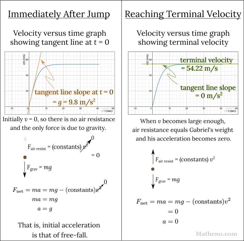
When a particular skydiver, Gabriel, jumps out of a plane at $𝑡 = 0$ , his velocity increases as shown in the graph below. At t = 41 seconds he deploys his parachute; we won't concern ourselves with what happens after that instant.

Graph of skydiver's velocity versus time. Starts at (0,0) and curves upward at a decreasing rate, leveling off at about t=16 seconds. There's an interactive version of the graph below.

a = 0 sec marks the beginning of the overall interval; b = 10 sec marks the end

We're going to determine how far Gabriel falls in the first 10 seconds of his jump — that is, from the start of the interval at $𝑎 = 0$ sec to $𝑏 = 10$ sec at the end of the interval.

Part I: 5-term approximation

To start, we'll use 5 subintervals, as shown in the figure, to approximate the distance he travels during these 10 seconds. Each subinterval thus has convenient duration $Δ 𝑡 = 10 s 5 = 2 s .$

Velocity versus time graph, now zoomed in to focus on the interval from t=0 to t=10 seconds. The graph also shows the n=5 subintervals from 0 to 2 sec, from 2 to 4 sec, and so forth

The animation to the right shows his 10-second fall broken in to the five 2-second intervals.

Let's quickly build our 5-term sums using this new notation.

Build the 5-term left sum

Let's compute the value of the left sum you just crafted as the 5-term underestimate: $Δ 𝑦 [0, 10] u n d e r e s t = 𝑆 𝐿 = 5 \sum 𝑖 = 1 𝑣 (𝑡 𝑖 - 1) \cdot Δ 𝑡 = 𝑣 (0) Δ 𝑡 + 𝑣 (2) Δ 𝑡 + 𝑣 (4) Δ 𝑡 + 𝑣 (6) Δ 𝑡 + 𝑣 (8) Δ 𝑡 = 0 \cdot 2 + 18.79 \cdot 2 + 33.55 \cdot 2 + 43.10 \cdot 2 + 48.52 \cdot 2 = 287.92 m ◂$

The 5-term overestimate for the distance Gabriel travels in the first 10 seconds of his fall is given by the right sum: $Δ 𝑦 [0, 10] o v e r e s t = 𝑆 𝑅 = 5 \sum 𝑖 = 1 𝑣 (𝑡 𝑖) \cdot Δ 𝑡 = 𝑣 (2) Δ 𝑡 + 𝑣 (4) Δ 𝑡 + 𝑣 (6) Δ 𝑡 + 𝑣 (8) Δ 𝑡 + 𝑣 (10) Δ 𝑡 = 18.79 \cdot 2 + 33.55 \cdot 2 + 43.10 \cdot 2 + 48.52 \cdot 2 + 51.38 \cdot 2 = 390.68 m ◂$ The error bound for our n = 5 subintervals is thus $e r r o r b o u n d = Δ 𝑦 [0, 10], o v e r e s t - Δ 𝑦 [0, 10], u n d e r e s t = 390.68 m - 287.92 m = 102.76 m ◂$ Said differently, we know the distance Gabriel falls in the first 10 seconds is bounded by $𝑆 𝐿 ⏞ 287.92 m \leq Δ 𝑦 [0, 10] \leq 𝑆 𝑅 ⏞ 390.68 m$

Part II: Focus on the error bound

Let's take a closer look at the calculation for the error bound, and develop a different way of determining how many terms n we need to use in our sum to achieve a particular tolerance. This approach only works in certain situations, as we'll see, but we think there's value in working a bit more with the left- and right- sums before we continue.

n = 5 terms

Let's first write out the sums for the overestimate and underestimate as above, but now with some added extra space and underlines to highlight a realization:

Δ 𝑦 o v e r e s t = 𝑆 𝑅 = 5 \sum 𝑖 = 1 𝑣 (𝑡 𝑖) \cdot Δ 𝑡 = 𝑣 (0) Δ 𝑡 + 𝑣 (2) Δ 𝑡 ――――― + 𝑣 (4) Δ 𝑡 ――――― ――――― + 𝑣 (6) Δ 𝑡 ――――― ――――― ――――― + 𝑣 (8) Δ 𝑡 ――――― ――――― ――――― ――――― + 𝑣 (10) Δ 𝑡 Δ 𝑦 u n d e r e s t = 𝑆 𝐿 = 5 \sum 𝑖 = 1 𝑣 (𝑡 𝑖 - 1) \cdot Δ 𝑡 = 𝑣 (0) Δ 𝑡 + 𝑣 (2) Δ 𝑡 ――――― + 𝑣 (4) Δ 𝑡 ――――― ――――― + 𝑣 (6) Δ 𝑡 ――――― ――――― ――――― + 𝑣 (8) Δ 𝑡 ――――― ――――― ――――― ―――――

Notice that most of the terms in the overestimate (right sum) and underestimate (left sum) are the same! Hence when we subtract the underestimate from the overestimate to find the error bound,

e r r o r b o u n d = Δ 𝑦 o v e r e s t - Δ 𝑦 u n d e r e s t

the $𝑣 (2) Δ 𝑡 ―――――$ terms cancel, as do the $𝑣 (4) Δ 𝑡 ――――― ―――――$ terms, and so forth. Indeed, the only terms that remain are the last term in the overestimate, $𝑣 (10) Δ 𝑡,$ and the first term in the underestimate, $𝑣 (0) Δ 𝑡$ :

e r r o r b o u n d = Δ 𝑦 o v e r e s t - Δ 𝑦 u n d e r e s t = [𝑣 (0) Δ 𝑡 + 𝑣 (2) Δ 𝑡 ――――― + 𝑣 (4) Δ 𝑡 ――――― ――――― + 𝑣 (6) Δ 𝑡 ――――― ――――― ――――― + 𝑣 (8) Δ 𝑡 ――――― ――――― ――――― ――――― + 𝑣 (10) Δ 𝑡] - [𝑣 (0) Δ 𝑡 + 𝑣 (2) Δ 𝑡 ――――― + 𝑣 (4) Δ 𝑡 ――――― ――――― + 𝑣 (6) Δ 𝑡 ――――― ――――― ――――― + 𝑣 (8) Δ 𝑡 ――――― ――――― ――――― ―――――] = 𝑣 (10) Δ 𝑡 - 𝑣 (0) Δ 𝑡 = (𝑣 (10) - 𝑣 (0)) \cdot Δ 𝑡, w h e r e Δ 𝑡 = 2 s

If we substitute the values

𝑣 (10) = 51.38 m s

and

𝑣 (0) = 0 m s

we find

e r r o r b o u n d = (51.38 - 0) \cdot 2 = 102.76 m ◂

which matches (as it must) the result we got above when we subtracted our underestimate of 287.92 m from the overestimate of 390.68 m.

In case you'd like a visual to see that the middle terms in the left and right sums are the same, drag the slider beneath this calculator all the way to the left. Since each rectangle represents one term in each sum, by comparing terms in this crafty way you can see how 4 of the 5 terms in each sum are actually the same.

Notice that with this new approach, we don't have to actually compute the sums to know what the error will be, which is rather remarkable: if you take the final velocity, subtract the initial velocity, and multiply by $Δ 𝑡,$ that tells you the error! This works because the function increases monotomically, and so the minimum velocity of each subinterval occurs at the interval's start (so the left sum is the underestimate) while the maximum occurs at the interval's end (so the right sum is the overestimate). We'll look later at non-monotonic functions where the min and/or max may occur somewhere other than the subinterval's endpoints, in which case the left and right sums do not necessarily yield a valid underestimate and overestimate.

But for now, we have a cool result for this situation that we're going to put to further use!

Generalize to any n terms

It probably won't surprise you that most of the terms cancel when we compute the error bound, no matter how many terms n there are. We'll show those cancellations in a minute. (Why, then, does the error decrease as n increases? Notice that $Δ 𝑡 = 10 s e c 𝑛 .$ We'll come back to this below.)

First, let's take this opportunity to generalize our indexing of the times we're using, $𝑡 0, 𝑡 1,$ and so on, up through $𝑡 𝑛,$ where n is still the number of intervals we're using. The slider beneath this calculator allows you to vary n, and you can see that each interval #i (starting with $𝑖 = 1$ ) begins at time $𝑡 𝑖 - 1$ and ends at time $𝑡 𝑖,$ up through time $𝑡 𝑛 .$ This may all seem straightforward and simple, and we hope that's the case; if so, you're doing great at tracking everything ('cause there's a lot going on here) and are largely ready for the big step we're going to take a few screens from now.

With our indexing in place, let's generalize the underestimate (left sum) and the overestimate (right sum) for n subintervals: $Δ 𝑦 o v e r e s t = 𝑛 \sum 𝑖 = 1 𝑣 (𝑡 𝑖) \cdot Δ 𝑡 = 𝑣 (𝑡 0) \cdot Δ 𝑡 + 𝑣 (𝑡 1) \cdot Δ 𝑡 ―――――― + 𝑣 (𝑡 2) \cdot Δ 𝑡 ―――――― ―――――― + \dots + 𝑣 (𝑡 𝑛 - 1) \cdot Δ 𝑡 ――――――― ――――――― ――――――― + 𝑣 (𝑡 𝑛) \cdot Δ 𝑡 Δ 𝑦 u n d e r e s t = 𝑛 \sum 𝑖 = 1 𝑣 (𝑡 𝑖 - 1) \cdot Δ 𝑡 = 𝑣 (𝑡 0) \cdot Δ 𝑡 + 𝑣 (𝑡 1) \cdot Δ 𝑡 ―――――― + 𝑣 (𝑡 2) \cdot Δ 𝑡 ―――――― ―――――― + \dots + 𝑣 (𝑡 𝑛 - 1) \cdot Δ 𝑡 ――――――― ――――――― ―――――――$ You can (and should) check for yourself that setting n = 5 in the preceding two lines reproduces the 5-term sums we developed just a little ways up the screen.

With the sums now generalized for any value of n, we can see that the same cancellations occur when we take the difference between the overestimate and underestimate, once again leaving only the last term of the overestimate and the first term of the underestimate: $e r r o r b o u n d = Δ 𝑦 o v e r e s t - Δ 𝑦 u n d e r e s t = [𝑣 (𝑡 0) \cdot Δ 𝑡 + 𝑣 (𝑡 1) \cdot Δ 𝑡 ―――――― + 𝑣 (𝑡 2) \cdot Δ 𝑡 ―――――― ―――――― + \dots + 𝑣 (𝑡 𝑛 - 1) \cdot Δ 𝑡 ――――――― ――――――― ――――――― + 𝑣 (𝑡 𝑛) \cdot Δ 𝑡] - [𝑣 (𝑡 0) \cdot Δ 𝑡 + 𝑣 (𝑡 1) \cdot Δ 𝑡 ―――――― + 𝑣 (𝑡 2) \cdot Δ 𝑡 ―――――― ―――――― + \dots + 𝑣 (𝑡 𝑛 - 1) \cdot Δ 𝑡 ――――――― ――――――― ―――――――] = 𝑣 (𝑡 𝑛) \cdot Δ 𝑡 - 𝑣 (𝑡 0) \cdot Δ 𝑡 = 𝑣 (𝑏) \cdot Δ 𝑡 - 𝑣 (𝑎) \cdot Δ 𝑡 [R e c a l l 𝑡 𝑛 = 𝑏, t h e i n t e r v a l' s e n d; 𝑡 0 = 𝑎, t h e i n t e r v a l' s s t a r t] = (𝑣 (𝑏) - 𝑣 (𝑎)) \cdot Δ 𝑡, w h e r e Δ 𝑡 = 𝑏 - 𝑎 𝑛 = 10 s 𝑛 ◂$ That last line also shows how the error bound decreases as $Δ 𝑡$ decreases: in this scenario the error bound is directly proportional to the subinterval width $Δ 𝑡!$

And $Δ 𝑡$ is inversely proportional to n. So as n increases, $Δ 𝑡$ decreases, as does the error bound.

$Δ 𝑡$ and n are inextricably linked

Indeed, this is a good time to start thinking of n and the interval width as being inextricably linked: $Δ 𝑡 = 𝑏 - 𝑎 𝑛$ Decreasing the subinterval size $Δ 𝑡$ (and hence the error bound) requires increasing the number of terms in the sum — because remember, all we're doing here is adding up (accumulating) the distance Gabriel falls in each subinterval i. And crucially

We can make the error bound arbitrarily close to zero
by making the width of each subinterval, $Δ 𝑡,$ sufficiently small.

Or, equivalently:

We can make the error bound arbitrarily close to zero
by making the number of subintervals, n, sufficiently large.

Let's put this result we've just developed for our scenario here $e r r o r b o u n d = (𝑣 (𝑏) - 𝑣 (𝑎)) \cdot Δ 𝑡$ to use.

Subinterval width, value of n, required for error bound of 4 meters

To determine the distance that Gabriel falls to within an error bound of 4 meters requires a minimum subinterval size of $Δ 𝑡$ = ____, which in turn requires n = ___ subintervals.

You can verify the answer you just found, and visualize using various number n of subintervals, using the calculator below.

As we conclude this screen, remember that we're using left and right sums to determine over- and underestimates because we know that the true value lies between the left and right sum values, and we can make the error bound as small as we'd like simply by increasing the number of subintervals that we use (or equivalently, by decreasing the subinterval width $Δ 𝑡$ ).

We can obtain an estimate for the distance Gabriel falls using other approaches as well. We'll introduce two of them on the next screen: midpoint sums, and trapezoidal sums. While perhaps not frequently used outside of classrooms, these two approaches appear routinely on exams, and also provide more practice with the ideas of developing net accumulation given a varying rate-of-change.

For now, what thoughts or questions do you have about what's on this screen? What other Calculus or Calculus-related questions do you have? Please let us know on the Forum!

The Upshot

To compute the distance an Gabriel falls given that his rate of travel varies, we use our usual approximation approach. We first break the overall motion into n subintervals, for instance $𝑛 = 5 .$ We then (1) approximate the distance Gabriel falls in each subinterval: $A p p r o x i m a t e Δ 𝑦 d u r i n g s u b i n t e r v a l 𝑖 : Δ 𝑦 𝑖 = (r e p r e s e n t a t i v e v e l o c i t y f o r t h i s s u b i n t e r v a l) \cdot (s u b i n t e r v a l d u r a t i o n)$ where the "representative velocity" we use is either his maximum velocity during that subinterval (which gives us an overestimate) or his minimum velocity during the subinterval (which gives us an underestimate). We then (2) sum $Δ 𝑦 𝑖$ for all of the subintervals: $Δ 𝑦 t o t a l = Δ 𝑦 1 + Δ 𝑦 2 + Δ 𝑦 3 + Δ 𝑦 4 + Δ 𝑦 5$ Our error bound is the difference between the overestimate and underestimate: we know that the true value lies somewhere between those two values.
We introduced some new notation: we use a to signify the beginning of the overall interval of interest (here, $𝑡 0 = 0$ seconds), and b to signify the end of the overall interval (here, $𝑡 𝑛 = 10$ seconds). Each subinterval then has width (time duration) $Δ 𝑡 = 𝑏 - 𝑎 𝑛 .$
To decrease the error bound, we increase the number n of subintervals in our calculation, thereby decreasing the subinterval width $Δ 𝑡 .$ We can make the error bound as small as we'd like by choosing n sufficiently large.