A.1 Context 1: Liquid Flow into, out of a Container

Here's a simple but important thing to say about integrals: they sum, or accumulate, what you put inside them. For instance, on this screen we will start to develop an integral that sums, or accumulates, the amount of liquid that flows into, and then out of, a container. The reason we need to develop the relevant integral is that we are given the rate at which the liquid flows, so rather than saying, for example, that "10 gallons of liquid enter," we are told that "liquid flows in at 6 gallons per minute," or that "liquid flows out at a rate that varies with time according to ....." As we'll see below and as we proceed, this is a classic case of needing an integral to complete the calculation we're after.

Note: This activity is based on work done by the CLEAR Calculus Project at Oklahoma State University. From the Project's website: "Project CLEAR Calculus is a research-based effort to make calculus conceptually accessible to more students while simultaneously increasing the coherence, rigor, and applicability of the content learned in the courses."
We at Matheno appreciate the work CLEAR Calculus has done to help students learn Calculus better, and are happy to build off of their efforts.

Photo of tall steel tank that can be filled and drained with liquid. — Cropped from Subhashish Panigrahi, CC BY-SA 4.0, via Wikimedia Commons.

Suppose we have a cylindrical storage tank that holds some liquid. Sometimes we're filling the tank; at other times, we drain it of the stored liquid.

Part I. Filling the tank at a constant rate

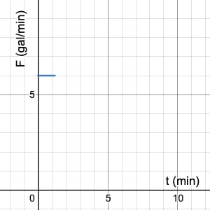
Let's start with the simplest case, in which we fill the tank at a constant flow rate F. Specifically, in this particular situation water flows into the tank at the constant flow rate of F = 6 gallons/minute.

Context 1 Warm-up Question

Given that the flow rate is $𝐹 = 6 g a l m i n$ , which graph correctly represents F versus time t?

(Click "Start graphs" below to see the answer choices.)

Now that we have a correct graphical representation of the rate at which we're filling the storage tank, let's consider the following question:

How much water accumulates over a given period of time,
given this constant rate of accumulation?

The answer may well be obvious to you, but we're going to build up slowly in order to extend step-by-step to more complicated scenarios from here.

Quick Calculation A: Water accumulated over 3 minutes

GIF of water filling a tank at a constant rate of 6 gallons per minute.

Play GIF

Let's start with this concrete and straightforward question: Given that the water flows in at the rate $𝐹 = 6 g a l m i n,$ how much water has accumulated in the tank after $Δ 𝑡 = 3$ minutes?

Solution.

Let's not over-complicate the required computation: If your intuition told you to simply multiply the rate and the time to find $A c c u m u l a t i o n o v e r 3 m i n u t e s = 6 g a l m i n \cdot 3 m i n = 18 g a l, ✓$ then you are absolutely correct. For the case of a constant rate-of-travel, you probably know the simple equation distance = rate • time. The same principle applies here; our rate just happens to be a fluid-flow-rate instead of a distance-rate.

For a visual of what's going on here, we can draw from the area model of multiplication. The animation may seem obvious, but please take the time to note what it shows because we'll be using more involved versions soon.

Quick Calculation B: Water accumulated over 5 minutes

Let's now extend the time interval of interest. The flowrate is again F = 6 gal/min. The amount of water that's accumulated after $Δ 𝑡 =$ 5 minutes is ___ gallons. (Please do the quick calculation to fill in that blank for yourself.)

Solution.You probably did the quick and correct calculation in your head: $6 g a l m i n \cdot 5$ min = 30 gallons. In and of itself, this result isn't very interesting.

Let's take this opportunity to shift our thinking to focus on what's happening in each 1-minute subinterval that passes: in each of those one minutes, we add 6 gallons to the tank. So after the full interval of 5 minutes, we have $A c c u m u l a t i o n o v e r 5 m i n u t e s = 5 t i m e s ⏞ ¯¯¯¯¯¯¯¯ ⏞ ¯¯¯¯¯¯¯¯ ⏞ 6 g a l + 6 g a l + 6 g a l + 6 g a l + 6 g a l = 30 g a l ✓$ The following animation illustrates this calculation — again, nothing surprising, but please take note of what it shows since we'll extend its use as we proceed.

Quick Calculation C: Water accumulated over 422 seconds

As a final calculation for this constant-rate filling with F = 6 gal/min, after $Δ 𝑡 =$ 422 seconds the amount of water in the tank is . . . . (Please either do the calculation, or at least think through what you'd enter into your calculator.)

Solution.To compute the requested value, we first need to convert the 422 seconds into minutes, since our flowrate is in gallons per minute. $Δ 𝑡 = 422 s e c \cdot 1 m i n 60 s e c = 42260 m i n = 21130 m i n = 7.0333 . . . = 7.0 ¯ 3 m i n$ (Recall that a number with a "bar" over it, like $¯ 3,$ means that that number repeats forever.)

Since our flow rate is $6 g a l m i n,$ the total accumulated water is 6 times as large: $= 6 g a l m i n \cdot 7.0 ¯ 3 m i n = 42.2 g a l ✓$ One way we can think of this is, as the animation shows, 6-gallons being accumulated 7 times, plus another 6 gallons $\cdot 0.0 ¯ 3 .$

Part II: Draining the tank with a changing flowrate

Imagine now that we want to transfer the liquid in the tank elsewhere, so we turn the source off and open the valve on the bottom of the tank. The liquid flows out and into another container where it accumulates.

It turns out that water doesn't drain out of its container at a constant rate. Instead, the flowrate-out depends on how much water is currently in the tank. Specifically, as you may have noticed, liquid drains out faster when a container is full (and there's a lot of volume pressing down on the liquid at the bottom that's about to leave), and more and more slowly as time passes and less liquid remains.

Rather than model this flowrate exactly, we're going to pretend that the flowrate decreases linearly with time according to the made-up equation $𝐹 (𝑡) = 6 - 90211 𝑡 [m a d e - u p f l o w r a t e f o r d r a i n i n g w a t e r]$ where t = 0 marks the moment we open the drain.

GIF of the flowrate equation F(t) = 6 - (90/211)t, showing a downward-sloped line.

Play GIF

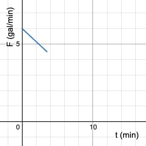
Note: Typically, flowrates into a tank are represented as positive values, while flowrates out of a tank are negative. Later we'll make use of this convention, but for now let's make this flowrate-out a positive value so we can focus on other key issues without the complication of negative signs on various values.

We're going to start to address a very similar question to the one we posed above:

How much water drains from the tank over time?

Specifically, we're going to work to determine how much water flows out of the tank in the 3 minutes after we open the drain. We'll refer to the amount of water that's drained out as an "accumulated value," which you can think of as either the sum of the water that has left the tank, or equivalently as the amount of water that is now in the other container to which it's been transferred.

Note: Depending on your experience in perhaps a previous Calculus or Physics class, you may immediately know how to calculate the value we're after here since the flowrate changes linearly. If so, we ask that you please pretend that you don't, and instead complete the calculations as we're laying them out. We purposefully started with a simple function so we can keep our focus on the new tools that we're going to be developing because, well, really they lie at the heart of integral Calculus. We know you want to understand deeply what an integral is all about, and building that understanding begins right here.

Question 1: Approach to calculate total waterflow out in 3 minutes

Two students discuss how to calculate how much water has left the tank after 3 minutes.

BANU: This is easy. Just like we did above, we can just multiply $6 g a l m i n \cdot 3 m i n$ to get 18 gallons drained from the tank.

NEVA: I don't think that's right, because the flowrate constantly changes. Multiplying $6 g a l m i n \cdot 3 m i n$ assumes that the flowrate is constant over that entire 3 minutes, but it isn't constant.

As Question 1 illustrates, since the flowrate changes as time passes, we can't do the same simple calculation we did above when the flowrate was constant. Instead we need to account somehow for the changing rate.

As a first step toward tackling this challenge, let's compute the flow rate at the times $𝑡 = 0,$ $𝑡 = 1$ minute, and $𝑡 = 2$ minutes. Recall that $𝐹 (𝑡) = 6 - 90211 𝑡,$ in gallons per minute. Hence $𝐹 (0) = 6 g a l m i n 𝐹 (1) = 6 - (90211) (1) = 1176211 = 5.573 g a l m i n 𝐹 (2) = 6 - (90211) (2) = 1086211 = 5.147 g a l m i n$

Question 2: Interpret F(1)

The two Questions above emphasize the point that the flowrate out of the tank changes continually, which means there is no obvious single value we can use as "the rate" over the entire 3-minute interval we're interested in.

The secret to Calculus: approximate to create a simpler problem.

But as we've seen time and again, we can make good progress by approximating the function's behavior with something simpler. And, what could be simpler than the calculations we did above in "Part I: Filling the tank at a constant rate"? Those calculations were so simple because the rate was constant, so let's adopt the same approach here and, for approximation purposes, replace our flowrate function with one that is constant over 1-minute subintervals. Specifically, we'll take the rate at the start of each 1-minute subinterval, its leftmost point, and pretend that the rate maintains that same value for the rest of that minute. The following animation illustrates.

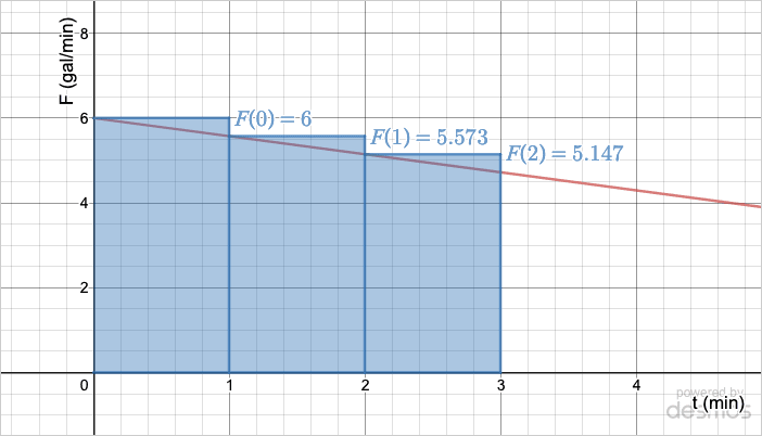
Graph of the flowrate out line, and the three rectangles overlaid, each spanning one minute. The first has height equal to F(0) = 6 and goes from t = 0 to 1 min. The second has height equal to F(1) = 5.573 and goes from t= 1 to 2 minutes. The third has height F(2) = 5.147 and goes from t = 2 to 3 minutes.

Using this approximation approach, our calculation is now simple: for each 1-minute subinterval, we can use our simple relation

accumulation = (rate at the start of the subinterval) • (subinterval length).

We then just add up what happens for each of the three minutes: $A p p r o x i m a t e a c c u m u l a t i o n = a c c u m f o r m i n 1 ⏞ ¯¯ ⏞ ¯¯ ⏞ 𝐹 (0) \cdot 1 m i n + a c c u m f o r m i n 2 ⏞ ¯¯ ⏞ ¯¯ ⏞ 𝐹 (1) \cdot 1 m i n + a c c u m f o r m i n 3 ⏞ ¯¯ ⏞ ¯¯ ⏞ 𝐹 (2) \cdot 1 m i n o v e r 3 m i n u t e s = 6 g a l m i n \cdot 1 m i n + 5.573 g a l m i n \cdot 1 m i n + 5.147 g a l m i n \cdot 1 m i n = 6 g a l + 5.573 g a l + 5.147 g a l = 16.72 g a l ✓$ To recap, for this approximation approach we measure the flowrate out of the tank at the beginning of every minute and use that value as the single constant rate over the entire 1-minute subinterval.

Left sum: use the function's value at each subinterval's leftmost point

Since for each subinterval we have used the flowrate function's value at the start, or left-most point, the quantity we computed is known as a left sum, which we denote $𝑆 𝐿 .$

Question 3: Overestimate or underestimate?

By using the first point in each 1-minute subinterval as the function's value for the entire 60 seconds means — for this particular decreasing linear function — that we're using the function's maximum value on the subinterval, which leads to the overestimate we found. Since this is an overestimate, we know that the true value must be less than our left-sum overestimate of 16.72 gallons: $A c t u a l a c c u m u l a t i o n o v e r 3 m i n u t e s < 𝑆 𝐿 ⏞ 16.72 g a l ✓$ Now, as we saw earlier in the course when we first calculated limits and then derivatives, bounding the actual value on only one side doesn't really help us much. Instead, of course we need to bound the actual value on the low end as well.

Calculating an underestimate

Our choice of using the first instant in each 1-minute subinterval to approximate the flowrate over the entire subinterval was actually arbitrary: we could have used the moment halfway through (t = 0.5 minutes, 1.5 minutes, and 2.5 minutes), or one-quarter of the way through, or.... Indeed, later we'll explore what happens when we make different choices to use as the representative value for each subinterval instead.

For now, we have a clear task at hand: we want to choose the point in the subinterval that has the minimum value. And for the actual flowrate function, the minimum value on each subinterval occurs . . . where?

Since our flowrate function is linear, the answer is easy to see: while the maximum value occurs at the start of the subinterval, the minimum value occurs at the end. That is, we pick the final, rightmost instant in each of our subintervals: $F o r t h e s u b i n t e r v a l [0, 1] w e u s e 𝑡 = 1 : 𝐹 (1) = 5.573 g a l m i n F o r t h e s u b i n t e r v a l [1, 2] w e u s e 𝑡 = 2 : 𝐹 (2) = 5.147 g a l m i n F o r t h e s u b i n t e r v a l [2, 3] w e u s e 𝑡 = 3 : 𝐹 (3) = 4.720 g a l m i n$ This approach assures that our approximated rate for each subinterval (the green horizontal lines in the figure) is less than or equal to the actual flowrate $𝐹 (𝑡)$ over that subinterval.

Graph of the flowrate out line, and the three rectangles overlaid, each spanning one minute. The first has height equal to F(1) = 5.573 and goes from t = 0 to 1 min. The second has height equal to F(2) = 5.147 and goes from t= 1 to 2 minutes. The third has height F(3) = 4.720 and goes from t = 2 to 3 minutes.

Our calculation is again simple: we're now simply using the rate at the end of each subinterval, so for every 1-minute we have "accumulation = (rate at the end of the subinterval) • (subinterval length)." As before, we then just add up what happens for each of the three minutes: $U n d e r e s t i m a t e a p p r o x = a c c u m f o r m i n 1 ⏞ ¯¯ ⏞ ¯¯ ⏞ 𝐹 (1) \cdot 1 m i n + a c c u m f o r m i n 2 ⏞ ¯¯ ⏞ ¯¯ ⏞ 𝐹 (2) \cdot 1 m i n + a c c u m f o r m i n 3 ⏞ ¯¯ ⏞ ¯¯ ⏞ 𝐹 (3) \cdot 1 m i n a c c u m u l a t i o n o v e r 3 m i n u t e s = 5.573 g a l m i n \cdot 1 m i n + 5.147 g a l m i n \cdot 1 m i n + 4.720 g a l m i n \cdot 1 m i n = 5.573 g a l + 5.147 g a l + 4.720 g a l = 15.44 g a l ✓$

Right sum: use the function's value at the subinterval's rightmost point

No surprise: since we are now using the flowrate function's value at the right-most point as the representative value in each subinterval, the quantity we just computed is known as a right sum, which we denote $𝑆 𝑅 .$

From our reasoning above we know that this right-sum value is a lower-bound to the amount of water actually drained over the 3 minutes: $𝑆 𝑅 ⏞ 15.44 g a l < A c t u a l a c c u m u l a t i o n o v e r 3 m i n u t e s$ Putting this together with the result we found above for the upper-bound of 16.72 gal, we have $𝑆 𝑅 ⏞ 15.44 g a l < A c t u a l a c c u m u l a t i o n o v e r 3 m i n u t e s < 𝑆 𝐿 ⏞ 16.72 g a l ✓$ Since we now know the true accumulation lies between those two values, we have an error bound (the difference between those values) of $e r r o r b o u n d = 16.72 g a l - 15.44 g a l = 1.28 g a l ◂$ That is, we know the true value to within 1.28 gallons. Now that error-size is rather large compared to a value that lies somewhere in the range 15.44 to 16.72 gallons . . . but we note that we're only using 3 subintervals to model the entire three minutes. You might have an idea for how we could make the approximations better. . . .

Before we start down that path, let's first stop and for a brief overview of what we've done so far. We'll be building up a lot of ideas in the coming screens, and want to make sure you're with us in developing these Big Ideas.

Overview of our approximation approach

Our approximation approach consists of two big steps to develop the overestimate of the accumulated amount of liquid:

Determine the overestimate for the amount accumulated in each 1-minute subinterval: $a m o u n t a c c u m u l a t e d o v e r t h i s 1 - m i n u t e s u b i n t e r v a l = (𝑚 𝑎 𝑥 r a t e o n t h i s s u b i n t e r v a l) \cdot (d u r a t i o n o f t h e s u b i n t e r v a l)$
Sum the overestimated amounts accumulated for the three 1-minute subintervals.

The approach for finding the underestimate is the same, except that in Step 1 we use the minimum rate instead of the maximum rate for each subinterval.

Integrals are sums of pieces of a something bigger

If you're thinking this seems straightforward, you are well on your way to understanding how integrals work. We'll let you in on the key understanding of integrals now: they are always a Sum of pieces of a bigger something. (As we'll see, that's why integrals are written with a big fancy "S," $\int$ : they are always a Sum.) The first step in developing an integral will always be to consider one component-part of that bigger thing, just as we've done here by looking at 1-minute subintervals of accumulation (the smaller bits) of the entire 3-minutes' accumulation we're interested in (the bigger thing).

Everything we do in this chapter will involve a Sum of something. The question you should always have in mind for yourself:

What is it that I'm summing here?

For now, let's try a practice problem that continues with 1-minute subintervals. Problems like this are common on exams.

Practice Problem #1: Lower bound on water drained (t = 3 to 7 min)

The table contains more values for the flowrate of water out of our container. Time t is given in minutes, while

𝐹 (𝑡)

is given in gal/min.

**Values for $𝐹 (𝑡)$**
t:	3	4	5	6	7	8
$𝐹 (𝑡)$ :	4.720	4.294	3.867	3.441	3.014	2.588

Given these values, the lower-bound on the actual amount of water that flows out between

𝑡 = 3

and

𝑡 = 7

minutes is

(A) 19.336 (B) 16.322 (C) 17.204 g a l (D) 14.616 (E) n o n e o f t h e s e

ABCDE

For problems like this one, we find a quick sketch of the graph extremely helpful to make it clear which values you should be using. Something as simple as sketch (a) on the left below does the job: clearly it's not numerically accurate, but it doesn't matter as long as its clear that the values decrease as time t increases. We've also indicated using brackets underneath the time interval of interest.

(a) Sketch of graph with time on the horizontal axis and flowrate on the vertical axis. Time tickmarks are labeled 1, 2, 3, ..., 8 min. Dots represent the values in the table: F(3) = 4.720 and so forth. While not numerically accurate, the dots desccend as you move to the right, indicating that the flowrate values decrease as the minutes pass. (b) Same graph, now with 4 rough rectangles sketched in for the 4 subintervals. The height of each equals the flowrate-value at the end of that subinterval.

Once we've sketched that, we can remind ourselves that the question is asking for the lower bound for the amount of water that flows during this interval, which means we should choose the minimum flowrate value for each of the four subintervals. For instance, when we think about drawing the rectangle for the first subinterval, from t = 3 to t = 4 minutes, we see we should use the value at the end of the interval, at its rightmost point,

𝐹 (4) = 4.294 g a l m i n .

Then the lower bound on the amount of water that flows out during that first minute is

u n d e r e s t f o r w a t e r t h a t f l o w s = 𝐹 (4) ⏞ ¯¯ ⏞ ¯¯ ⏞ (4.294 g a l m i n) \cdot (1 m i n) f r o m 𝑡 = 3 \to 𝑡 = 4 m i n

Proceeding similarly for all four rectangles gives us the total underestimate for the water that flows from

𝑡 = 3

𝑡 = 7

minutes using the right sum:

u n d e r e s t = 𝑆 𝑅 = 𝐹 (4) ⏞ ¯¯ ⏞ ¯¯ ⏞ (4.294 g a l m i n) \cdot (1 m i n) + 𝐹 (5) ⏞ ¯¯ ⏞ ¯¯ ⏞ (3.867 g a l m i n) \cdot (1 m i n) + 5555555555 𝐹 (6) ⏞ ¯¯ ⏞ ¯¯ ⏞ (3.441 g a l m i n) \cdot (1 m i n) + 𝐹 (7) ⏞ ¯¯ ⏞ ¯¯ ⏞ (3.014 g a l m i n) \cdot (1 m i n) = 14.616 g a l ⟹ (D) ✓

The graph below is a nicer representation of the calculation. Graph showing underestimate rectangles

[close solution]

Practice Problem #2: Upper bound on water drained (t = 3 to 7 min)

The table contains values for the flowrate of water out of our container, repeated from the preceding problem. t is again given in minutes, while

𝐹 (𝑡)

is given in gal/min.

**Values for $𝐹 (𝑡)$**
t:	3	4	5	6	7	8
$𝐹 (𝑡)$ :	4.720	4.294	3.867	3.441	3.014	2.588

Given these values, the upper-bound on the actual amount of water that flows out between

𝑡 = 3

and

𝑡 = 7

minutes is

(A) 19.336 (B) 16.322 (C) 17.204 g a l (D) 14.616 (E) n o n e o f t h e s e

ABCDE

For additional practice, let's apply the same ideas to a different scenario.

Practice Problem #3: Left sum — students entering the auditorium

Monotonically increasing function of R versus t. Necessary values from the graph are stated in the accompanying table.

The rate at which students enter a large auditorium is given by

𝑅 (𝑡),

is shown in the graph to the right. Selected values for the rate are in the table for your convenience. For instance, at

𝑡 = 20

minutes, the rate at which students enter the auditorium is 27 students per minute.

t [minutes]	0	5	10	15	20	25	30	35
$𝑅 (𝑡)$ [students per minute]	7	8	10	14	27	38	41	42

Use a Left Sum with three subintervals to approximate the number of students who enter the auditorium from

𝑡 = 0

𝑡 = 30

minutes.

(A) 387 s t u d e n t s (B) 433 s t u d e n t s (C) 440 s t u d e n t s

(D) 615 s t u d e n t s (E) 1320 s t u d e n t s

ABCDE

Practice Problem #4: Right sum — students entering the auditorium

As in the preceding problem, the rate at which students enter a large auditorium is given by

𝑅 (𝑡),

as shown both in the graph and in the table below.

t [minutes]	0	5	10	15	20	25	30	35
$𝑅 (𝑡)$ [students per minute]	7	8	10	14	27	38	41	42

Use a Right Sum with three subintervals to approximate the number of students who enter the auditorium from

𝑡 = 0

𝑡 = 30

minutes.

(A) 530 s t u d e n t s (B) 780 s t u d e n t s (C) 890 s t u d e n t s

(D) 1200 s t u d e n t s (E) 2340 s t u d e n t s

ABCDE

Before we leave this screen, let's step back to take an overview of what the process we're now using. As we did earlier in the course, we'll use our Questions for Approximations to frame our work. Use the work we did above to answer these questions for yourself before revealing our answers.

Questions for Approximations [Reference]

1. What are you approximating? Why can't you find the exact value immediately?

2. How do you generate an overestimate for the value we're after? An underestimate?

We'll focus more on the remaining two questions in a bit. For now, as a reminder they are:

3. What is the difference between your current overestimate and underestimate values is your "error bound." What is its current value?

We calculated this value for our interval of $𝑡 = 0$ to $𝑡 = 3$ minutes above. We're not so interested in the exact number at this point; it's enough to know we can calculate it once we have the overestimate and underestimate.

4. How can the error bound be made smaller than any predetermined value?

We'll see in a few screens how the magic of Calculus answers this question! (And you may well already have your own answer in mind....)

The Upshot

Calculating the amount of "stuff" accumulated over a subinterval is completely straightforward if the accumulation-rate is constant:
accumulation = (constant rate) • (interval length)
When a rate changes from moment to moment (i.e., is not constant), we can approximate the actual total accumulation by (1) using a constant rate over each smaller subinterval to approximate the accumulation during that single subinterval, and then (2) summing those subinterval approximations to approximate the total value.
The approximations for these smaller, bit-by-bit accumulations can be visualized on a graph as rectangles, since they are calculated by multiplying the function's representative value (the height of the rectangle) by the subinterval's duration (the rectangle's width).
If we use the function's value at the start of each subinterval, at its leftmost point, we are computing a left sum, $𝑆 𝐿 .$ Similarly, if we use the function's value at the end of each subinterval, at its rightmost point, we are computing a right sum, $𝑆 𝑅 .$

We're well on our way to developing a strong understanding of what an integral is. We'll continue that development on the coming screens, starting on the next where we'll review (or perhaps introduce) how to use sigma notation, like $𝑛 \sum 𝑖 = 1,$ to convey a lot of information compactly. As we said above, integrals are sums, and in fact the integral is defined by a sum using sigma notation, so we need to be sure that you understand the notation completely. (Plus it's kinda fun.)

For now, there are already some Big Ideas on this screen. What questions or thoughts do you have? Please head over to the Forum and let us know!

Reference for Oehrtman's Five Questions: Oehrtman, M. (2008). Layers of abstraction: Theory and design for the instruction of limit concepts. In M. P. Carlson & C. Rasmussen (Eds.), Making the Connection: Research and Teaching in Undergraduate Mathematics Education, (MAA Notes, Vol. 73, pp. 65-80). Washington, DC: Mathematical Association of America.

A.1 Context 1: Liquid Flow into, out of a Container

Part I. Filling the tank at a constant rate

Part II: Draining the tank with a changing flowrate

Calculating an underestimate

Overview of our approximation approach

The Upshot

How helpful was this page?