A.5 Midpoint & Trapezoidal Sums

On this screen we introduce the midpoint sum, and the trapezoidal sum. We'll use each to estimate the distance Gabriel falls during the first ten seconds of his skydiving jump (introduced on the preceding screen). We won't do much with these two approximation methods beyond introducing them here and providing practice problems (of course), but since they appear frequently on exams you should absolutely know how to compute them. (As a side note, the name "trapezoidal sum" is potentially quite misleading for reasons we'll see below.)

Both methods start with the same basic approach we've been using. Specifically, to approximate the total distance Gabriel falls in the 10 seconds we:

1. Approximate the distance Gabriel falls in each subinterval:

A p p r o x i m a t e Δ 𝑦 d u r i n g s u b i n t e r v a l 𝑖 : Δ 𝑦 𝑖 = (r e p r e s e n t a t i v e v e l o c i t y f o r t h i s s u b i n t e r v a l) \cdot (s u b i n t e r v a l d u r a t i o n)

2. Sum $Δ 𝑦 𝑖$ for all of the subintervals:

Δ 𝑦 t o t a l = Δ 𝑦 1 + Δ 𝑦 2 + Δ 𝑦 3 + Δ 𝑦 4 + Δ 𝑦 5

The only new bit on this screen are two different values we can use as the representative velocity in step 1, which lead to (I) the midpoint sum and (II) the trapezoidal sum. Both of these approaches have the advantage that they typically give a more accurate approximation than does either the right or left sums alone for a given number of subintervals, like n = 5.

On the other hand, these two approaches do not let us visualize the associated error as easily as we can when we bound the true value by the overestimate and underestimate as we have been. Recall that with our previous approach, in which we find both an underestimate and an overestimate, we are assured that the true value likes somewhere between those two values, and we can easily calculate the current error bound for the n subintervals we are using. By contrast here, while we can still make the error smaller by increasing the number of subintervals, and equivalently decreasing the subintervals' duration, calculating the error means invoking a formula (that we're not including here) that doesn't offer us the same insights.

Expect these exam questions

You should expect exam questions in which you're asked to compute both the midpoint and trapezoidal sums, along with the left and right sums we introduced earlier. As you become familiar with the calculations here, you'll see that these problems are pretty routine (if tedious).

Recall the skydiver's velocity versus time graph from the preceding screen that we're using as our example here:

Velocity versus time graph, now with n = 5 subintervals from t-sub-a = 0 sec to t-sub-b = 10 sec. The endpoints of the subintervals are marked: t-sub-a = t-sub-0 = 0 s, t-sub-1 = 2 s, t-sub-2 = 4 s, t-sub-3 = 6 s, t-sub-4 = 8 s, and t-sub-b = t-sub-5 = 10 s.

We'll first examine the midpoint sum, using the same n = 5 subintervals as we did initially on the preceding screen.

Midpoint sums (use arithmetic mean of input values)

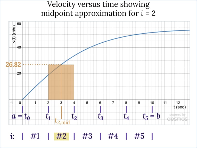
The idea behind the midpoint sum, $𝑆 m i d,$ is straightforward: rather than computing the fuction's representative value at either the start (left) or the end (right) of the interval, we compute the function's value at the interval's midpoint, halfway between the subinterval's beginning and end input-values:

DEFINITION

Midpoint sum

The midpoint sum is a Riemann sum that uses the arithmetic mean of the input values for each subinterval as the representative value.

𝑡 m i d = 𝑡 𝑖 - 1 + 𝑡 𝑖 2

M i d p o i n t a p p r o x i m a t i o n f o r s u b i n t e r v a l 𝑖 : Δ 𝑦 𝑖, m i d = (v e l o c i t y a t 𝑖' s m i d p o i n t) \cdot (s u b i n t e r v a l d u r a t i o n) = 𝑣 (𝑡 m i d) \cdot Δ 𝑡

Notice that in this approach, we take the arithmetic mean of the input values for this subinterval, and then use the velocity at that midpoint-instant as our representative value.

For instance, as you can see in the figure for 4th subinterval, i = 4, between t = 6 sec and t = 8 sec, we use the function's value at $𝑡 4, m i d = 7$ sec as its representative value for the interval.

Same graph, for the midpoint sum now showing an orange rectangle with base from t = 6 sec to t = 8 sec, and height equal to v(7). Text says that in the midpoint approximation for subinterval #4 from t = 6 s to t = 8 s, we use the input value halfway between the subinterval's endpoints, t-sub-4,mid = (t-sub-3 + t-sub-4) divided by 2 equals (6 sec + 8 sec) divided by 2 equals 14 sec divided by 2 equals 7 sec.

Let's try a practice problem.

Practice Problem #1

Gabriel's velocity at 1-second intervals
t (s)	0	1	2	3	4	5	6	7	8	9
$𝑣 (𝑡)$ (m/s)	0	9.69	18.79	26.82	33.55	38.94	43.10	46.22	48.52	50.19

The table provides Gabriel's velocity at 1-second intervals. (These values are from Gabriel's velocity versus time graph.) Use the data to find

Δ 𝑦 [2, 4] m i d

, the midpoint approximation for the distance Gabriel travels from t = 2 s to t = 4 s.

(A) 26.82 m (B) 37.58 m (C) 53.64 m (D) 67.10 m (E) n o n e o f t h e s e

ABCDE

Developing the midpoint sum for n = 5

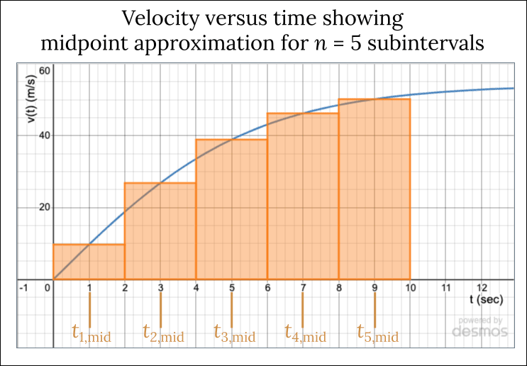
Same graph, now showing the 5 rectangles for the n=5 subintervals. Each is again 2 seconds in width, and the height of each equals the velocity at the midpoint of the subinterval.

To compute the midpoint approximation for the entire distance Gabriel falls during the 10 seconds, we continue with the approach you used in Problem #1: as shown in the figure, we use the value of the velocity at the midpoint of each subinterval. Hence we use for subinterval i = 1 the time $𝑡 1, m i d = 1$ s; $𝑡 2, m i d = 3$ s, and so forth, through $𝑡 5, m i d = 9$ s. We can use the data from the table in Problem 1, or the graph, to find the relevant velocity values. Then summing what happens over the 5 subintervals gives us $Δ 𝑦 [0, 10], m i d = 𝑆 m i d = Δ 𝑦 1, m i d + Δ 𝑦 2, m i d + Δ 𝑦 3, m i d + Δ 𝑦 4, m i d + Δ 𝑦 5, m i d = 𝑣 (1) \cdot Δ 𝑡 + 𝑣 (3) \cdot Δ 𝑡 + 𝑣 (5) \cdot Δ 𝑡 + 𝑣 (7) \cdot Δ 𝑡 + 𝑣 (9) \cdot Δ 𝑡 = 9.69 m s \cdot (2 s) + 26.82 m s \cdot (2 s) + 38.94 m s \cdot (2 s) + 46.22 m s \cdot (2 s) + 50.19 m s \cdot (2 s) = 343.72 m ◂$ Note that, as we would expect, this value lies between the under- and overestimates that we calculated on the previous screen for n = 5 subintervals: $287.92 m \leq Δ 𝑦 [0, 10], m i d \leq 390.68 m .$

Generalizing the midpoint sum for any n

We can of course again make the subinterval width $Δ 𝑡$ as small as we'd like by making the number of subintervals n sufficiently large. To do so, we first need to write the representative time for each subinterval, $𝑡 𝑖, m i d,$ in terms of i. A little thought shows that $𝑡 𝑖, m i d = (𝑖 - 12) Δ 𝑡 ◂$ You can check this against the values of $𝑡 𝑖, m i d$ we used above for n = 5 (and hence $Δ 𝑡 = 2$ s): $𝑡 1, m i d = 1$ s, $𝑡 2, m i d = 3$ s, and so forth.

The midpoint approximation sum is then given by $Δ 𝑦 [0, 10], m i d = 𝑆 m i d = 𝑛 \sum 𝑖 = 1 𝑣 (𝑡 𝑖, m i d ⏞ ¯¯ ⏞ ¯¯ ⏞ (𝑖 - 12) Δ 𝑡) \cdot Δ 𝑡, w h e r e Δ 𝑡 = 10 s 𝑛$ You can again check this sigma-notation version of the sum with the terms we've written out for n = 5 above.

When you're ready, you can use the slider beneath the following calculator to vary n and see the new sum that results. Crucially, notice that no matter how small the width, the height of each rectangle always equals the value of the velocity at the midpoint of its subinterval.

Notice once again that while we can easily obtain a value for the midpoint sum, we have no immediate information about how close it is to the true distance Gabriel falls.

We'll provide some practice at computing midpoint sums below. Before then, let's look at trapezoidal approximations.

Trapezoidal Approximations (use arithmetic mean of output values)

Recall that on the previous screens, we developed one estimated value by computing the left sum using the function's value at the leftmost point of each subinterval, and a second estimate by computing the right sum using the rightmost point. We can instead obtain a single estimate by combining these two approaches: for the function's representative value, we use the arithmetic mean of the function's output values at the leftmost and rightmost points:

DEFINITION

Trapezoidal sum

The trapezoidal sum is a Riemann sum that uses the arithmetic mean of the output values for each subinterval as the representative value.

r e p r e s e n t a t i v e v e l o c i t y d u r i n g s u b i n t e r v a l 𝑖 : 𝑣 𝑖, a v g = 𝑣 (𝑡 𝑖 - 1) + 𝑣 (𝑡 𝑖) 2

Hence the trapezoidal approximation for the subinterval is given by

T r a p e z o i d a l a p p r o x i m a t i o n f o r s u b i n t e r v a l 𝑖 : Δ 𝑦 𝑖, t r a p = (𝑣 𝑖, a v g) \cdot (s u b i n t e r v a l d u r a t i o n) = (𝑣 (𝑡 s u b i n t e r v a l s t a r t) + 𝑣 (𝑡 s u b i n t e r v a l e n d) 2) \cdot (s u b i n t e r v a l d u r a t i o n)

For instance, as you see in the figure, for subinterval i = 4 (t = 6 to 8 sec) we use as the representative velocity the arithmetic mean of the velocities at the start (t = 6 sec) and end (t = 8 sec) of the subinterval.

Developing the trapezoidal sum for n = 5

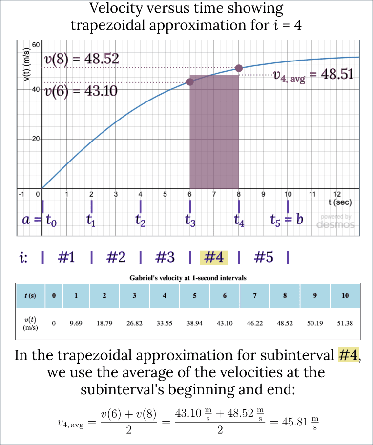
Velocity versus time graph showing rectangle for subinterval i = 4, so the base again goes from t = 6 sec to t = 8 sec. Labeling indicates the velocity at the subinterval's start, v(6), and at the subinterval's end, v(8). The height of the rectangle equals the arithmetic mean of those two values: v(6) plus v(8), all divided by 2.

Let's write out the n = 5 terms for Gabriel's travel over the 10 seconds using the trapezoidal approximation. Once again, $Δ 𝑡 = 10 s 5 = 2 s .$ Then the trapezoidal sum, $𝑆 t r a p,$ is

Δ 𝑦 [0, 10], t r a p = 𝑆 t r a p = 𝑖 = 1 ⏞ ¯¯¯ ⏞ ¯¯¯ ⏞ 𝑣 (0) + 𝑣 (2) 2 \cdot Δ 𝑡 + 𝑖 = 2 ⏞ ¯¯¯ ⏞ ¯¯¯ ⏞ 𝑣 (2) + 𝑣 (4) 2 \cdot Δ 𝑡 𝑚 𝑚 𝑚 + 𝑖 = 3 ⏞ ¯¯¯ ⏞ ¯¯¯ ⏞ 𝑣 (4) + 𝑣 (6) 2 \cdot Δ 𝑡 + 𝑖 = 4 ⏞ ¯¯¯ ⏞ ¯¯¯ ⏞ 𝑣 (6) + 𝑣 (8) 2 \cdot Δ 𝑡 + 𝑖 = 5 ⏞ ¯¯¯ ⏞ ¯¯¯ ⏞ 𝑣 (8) + 𝑣 (10) 2 \cdot Δ 𝑡

We can save ourselves a little computational work if we combine some terms. For instance, looking at the first two terms of the sum (for i = 1 and 2) we see that there's a $𝑣 (2)$ in both; in the second and third terms there's a $𝑣 (4)$ in both, and so on. Let's also factor out the $Δ 𝑡$ from all of the terms. We can thus rewrite our equation as

Δ 𝑦 [0, 10], t r a p = [12 𝑣 (0) + 𝑣 (2) + 𝑣 (4) + 𝑣 (6) + 𝑣 (8) + 12 𝑣 (10)] \cdot Δ 𝑡

Finally we substitute values to find the sum:

Δ 𝑦 [0, 10], t r a p = [12 \cdot 0 m s + 18.79 m s + 33.55 m s + 43.10 m s + 48.52 m s + 12 \cdot 51.38 m s] \cdot (2 s) = 339.30 m ◂

Ah, and we notice that once again as we expect, this value lies between the under- and overestimates that we calculated on the previous screen forn = 5 subintervals: $287.92 m \leq Δ 𝑦 [0, 10], t r a p \leq 390.68 m .$

Generalizing the trapezoidal sum for any n

We're actually not going to develop this fully using sigma notation. You can certainly imagine what the steps would be, and see how we'd write $𝑣 (𝑡 s u b i n t e r v a l s t a r t) = 𝑣 ((𝑖 - 1) Δ 𝑡)$ and $𝑣 (𝑡 s u b i n t e r v a l e n d) = 𝑣 (𝑖 Δ 𝑡),$ and so on.

Instead, recall the expression we developed above for the trapezoidal approximation to the distance Gabriel falls with $𝑛 = 5 :$ $Δ 𝑦 [0, 10], t r a p = [12 𝑣 (0) + 𝑣 (2) + 𝑣 (4) + 𝑣 (6) + 𝑣 (8) + 12 𝑣 (10)] \cdot Δ 𝑡$ Notice that, as we discussed above, the first and last terms have a factor of $12$ in front, while none of the terms "in the middle" do. We can extend this result to any number of terms, and write that for any number n of subintervals:

DEFINITION

Trapezoidal Approximation

Δ 𝑦 [0, 10], t r a p = 𝑆 t r a p = [12 𝑣 (𝑎) + 𝑣 (𝑡 1) + 𝑣 (𝑡 2) + \dots + 𝑣 (𝑡 𝑛 - 1) + 12 𝑣 (𝑏)] \cdot Δ 𝑡

where $𝑡 = 𝑎$ marks the start of the subinterval, $𝑡 = 𝑏$ marks the end of the subinterval, and $Δ 𝑡 = 𝑏 - 𝑎 𝑛 .$

As we wrote above for the midpoint sum, if you get a homework or exam question requesting a trapezoidal approximation, we strongly suggest making a table or using the one provided, and then just remember that the first and last values for the subinterval get that factor of $12$ while the other "middle" terms do not. (And of course don't forget to multiply everything by the subinterval width, $Δ 𝑡 .$ )

We're not doing more here because we won't discuss the Trapezoidal approximation again, whereas we will proceed with the left, right, and midpoint sums on the next screen. We're eager to get there because that's going to be a big step toward developing integrals.

Do please be sure to practice the problems below, and in later review sections. As we've said a few times now, you absolutely should expect exam questions that use the left, right, midpoint and trapezoidal approximations.

The name "Trapezoidal Approximation"

Before we leave this topic, let's address the name "Trapezoidal Approximation." We've emphasized that this approach uses the arithmetic mean of the function's output values as the representative value for Gabriel's velocity over each subinterval. We like this way of thinking about the method because it's easy to remember, and we can easily reconstruct the necessary calculations we need from this single idea. The graph on the left in the figure below replicates the one above as a reminder of the calculation we did. If you keep this picture in mind, you will never go wrong.

Left figure duplicated from the calculation above for the trapezoidalsum approximation for i=4, between t = 6 and 8 seconds. The height of the rectangle is the arithmetic mean of the velocities at the start and end of the interval, (1/2)*[v(6) + v(8).] Figure on the right showns the same graph with the same subinterval highlighted, but now a trapezoid instead: the width is still delta-t = 2 seconds, the left side has height equal to v(6), and the right has height equal to v(8). Text says that the area of the rectangle on the left, and of the trapezoid on the right, are equal: A = (1/2)[v(6 + v(8)] * delta-t.

Alternatively, we can view the calculation, as most textbooks do, as finding the area of the trapezoid shown in the right graph above. Note that the top of the trapezoid is formed by the (tilted) line segment that joins the left and right points of the subinterval. One way to think about formula for the trapezoid's area is that the factor of $12$ comes from the fact that the average height of the trapezoid is $12 [(l e f t s i d e h e i g h t) + (r i g h t s i d e h e i g h t)] .$ The areas of the rectangle on the left and the trapezoid on the right are thus the same.

You can of course choose to think of whichever figure works best for you, and we encourage you to do so! (That said, if you're curious about why the name "trapezoidal approximation" is potentially misleading and may get you into trouble, read on.)

The Upshot

Midpoint and trapezoidal sums still use the basic formulation (1) approximate the distance Gabriel falls in each subinterval: $A p p r o x i m a t e Δ 𝑦 d u r i n g s u b i n t e r v a l 𝑖 : Δ 𝑦 𝑖 = (r e p r e s e n t a t i v e v e l o c i t y f o r t h i s s u b i n t e r v a l) \cdot (s u b i n t e r v a l d u r a t i o n)$ and then (2) sum $Δ 𝑦 𝑖$ for all of the subintervals: $Δ 𝑦 t o t a l = Δ 𝑦 1 + Δ 𝑦 2 + Δ 𝑦 3 + Δ 𝑦 4 + Δ 𝑦 5$ The only new piece is the "representative velocity" we use for each subinterval:
For the midpoint sum, we focus on the input value and use the function's value at the midpoint of the interval, $𝑡 𝑖, m i d = 𝑡 𝑖 - 1 + 𝑡 𝑖 2 .$ That is, we take as the representative value $𝑣 𝑖 (𝑡 𝑖, m i d) .$
For the trapezoidal sum, we focus on the output value and use the arithmetic mean of the function's output values at the left and right endpoints: $𝑣 𝑖, a v g = 𝑣 (𝑡 𝑖 - 1) + 𝑣 (𝑡 𝑖) 2 .$

On the next screen we're going to introduce (yet) two more types of approximation sums that are fundamentally important.

For now, are Midpoint Sums and Trapezoidal Sums making sense to you? Are you trying to use them in an unfamiliar context? Let us know what questions you have on the Forum, and we'll do our best to assist!

A.5 Midpoint & Trapezoidal Sums

Midpoint sums (use arithmetic mean of input values)

Developing the midpoint sum for n = 5

Generalizing the midpoint sum for any n

Trapezoidal Approximations (use arithmetic mean of output values)

Developing the trapezoidal sum for n = 5

Generalizing the trapezoidal sum for any n

The name "Trapezoidal Approximation"

The Upshot

How helpful was this page?