B.2 Average Velocity Over Any Interval

On the preceding screen we developed the concept of "average velocity for an entire trip." On this screen we're going to extend those ideas to apply to the average velocity over any time interval that we choose. We'll then take a very big step, and start to develop the idea of instantaneous velocity.

Average velocity: average rate of change of position over a specified time interval

The only change from the preceding screen is that, no surprise, instead of considering the entire trip, we instead must specify the exact time interval we're interested in. We use the notation $𝑡 1$ to specify the start of the interval, and $𝑡 2$ to specify its end; the time interval is thus $[𝑡 1, 𝑡 2] .$ We also need to know the object's position at the start of the interval $𝑠 (𝑡 1),$ and its position at the end of the interval, $𝑠 (𝑡 2) .$

We can then generalize average velocity over any interval as

DEFINITION

Average velocity over any interval

a v e r a g e v e l o c i t y [𝑡 1, 𝑡 2] = c h a n g e i n p o s i t i o n c h a n g e i n t i m e = f i n a l p o s i t i o n - i n i t i a l p o s i t i o n f i n a l t i m e - i n i t i a l t i m e = 𝑠 (𝑡 2) - 𝑠 (𝑡 1) 𝑡 2 - 𝑡 1

We use the subscript $[𝑡 1, 𝑡 2]$ on the words "average velocity" to emphasize that we are computing the average rate of change of the object's position over this particular time interval from $𝑡 1$ to $𝑡 2,$ so it's perfectly clear to anyone looking at the calculation what the relevant interval is.

In the following Example, let's compute the average velocity for an interval that does not encompass the entire trip.

Example 1: Samuel's Average Velocity

Samuel's position as a function of time for a trip is shown below. Each position is a mile-marker along the highway.

t i m e p o s i t i o n 2 : 00 p m 130 2 : 20 p m 107 2 : 40 p m 89 3 : 00 p m 75 3 : 20 p m 68 3 : 40 p m 68 4 : 00 p m 42 4 : 20 p m 28 5 : 00 p m 10

What was his average velocity between 3:00 pm and 4:20 pm?
The answer is a negative value. What's the physical significance of this negative result?

Solution.

(a) Samuel's average velocity between 3:00 pm and 4:20 pm is

a v e r a g e v e l o c i t y [3 : 00 p m, 4 : 20 p m] = 𝑠 (4 : 20 p m) - 𝑠 (3 : 00 p m) 4 : 20 p m - 3 : 00 p m = 28 m i l e s - 75 m i l e s 1 h o u r 20 m i n = - 47 m i l e s 1.33 h o u r s = - 35.3 m p h ✓

(b) As the figure below shows, the negative value indicates that Samuel's final position, s(4:20 pm) = 28 miles, is closer to the origin than his initial position, s(3:00 pm) = 75 miles. That is, his position has decreased over this interval. The line segment connecting his initial and final positions thus has a negative slope. Samuel's position versus time graph, with a line secant passing through the points (3:00pm, mile 75) and (4:20pm, mile 28), marking the start and end of the interval. The slope of that line equals Samuel's average velocity over the interval, and is negative because his position decreases over the interval.

Samuel's position versus time graph, with a line secant passing through the points (3:00pm, mile 75) and (4:20pm, mile 28), marking the start and end of the interval. The slope of that line equals Samuel's average velocity over the interval, and is negative because his position decreases over the interval.

Thinking about short time intervals,
and initial "instantaneous velocity" estimates

We're now making a Big Shift, and starting to think about what happens over as short a time interval as we can compute with the data we are given, around a particular moment. For instance, in the following Example we'll estimate the "instantaneous velocity" at a particular time — that is, approximately what a car's speedometer would show at that instant.

This Example, by the way, is based on a very common exam question, so you should become comfortable with it, along with the other similar Examples and Practice Problems below.

Example 2: Approximate an object's velocity at an instant

A remote-controlled toy car travels on a straight track, starting from position s = 0 at time t = 0. Its position at time t is given by the function $𝑠 (𝑡) .$ The table shows values of its position, measured in centimeters (cm), at some moments in time, measured in seconds from $𝑡 = 0 .$

$𝑡 (s e c o n d s) 1.0 1.5 3.0 3.5 4.0 4.5 𝑠 (c m) 1.0 2.25 9.0 12.25 16 20.25$

Graph showing data points listed in the table

The data points are plotted in the figure.

Use two of the data points given to approximate as best you can the object's velocity at $𝑡 = 3.0$ seconds.

Solution.

We can't use only the data point for $𝑡 = 3.0$ s to find the car's velocity at that instant: that single piece of information tells us where the object is just then, but not how fast it's moving. Instead, to find its velocity we need to compute its change in position over some time interval.

To get the best approximation we can using the given data, we should take the smallest time interval we can near $𝑡 = 3.0$ s. There's no sense, for instance, in computing the average velocity over the entire period [1.0 s, 4.5 s]: the value we would obtain is unlikely to accurately represent what happens at t = 3.0 s.

By contrast, the data point at $𝑡 = 3.5$ s is just 0.5 s away from our moment of interest, and the interval [3.0 s, 3.5 s] is only 0.5 s long. So let's use the data points for those two times: $𝑡 (s e c o n d s) 1.0 1.5 3.0 3.5 4.0 4.5 𝑠 (c m) 1.0 2.25 9.0 12.25 16 20.25$ That is, let's use the points (3.0, 9) and (3.5, 12.25) to find the average velocity over that 0.5-second interval, and take that the resulting value as the best possible approximation to the velocity at t = 3.0 s we're after.

Recall the definition of average velocity: $a v e r a g e v e l o c i t y [3.0, 3.5] = 𝑠 (𝑡 2) - 𝑠 (𝑡 1) 𝑡 2 - 𝑡 1 = 𝑠 (3.5) - 𝑠 (3.0) 3.5 - 3.0 = 12.25 - 9.0 0.5 = 3.25 0.5 = 6.5 c m / s$

Graph showing data points listed in the table and the secant line through the two points of interest. The slope of that secant line equals the average velocity for the interval, 6.5 m/s.

The average velocity we just calculated is equal to the slope of the secant line that passes through the points $(3.0, 𝑠 (3.0))$ and $(3.5, 𝑠 (3.5)),$ as shown.

The preceding examples used tables to provide the position-values at various times. More frequently, you'll be given an equation that describes an object's position as a function of time, and your first step will be to use that equation to determine the object's position final and initial positions for the interval of interest. Example 3 illustrates.

Example 3: Ball Tossed in the Air

A ball is shot from the ground straight up into the air with a velocity of $15 m / s .$ Its height is described by $𝑦 (𝑡) = 15 𝑡 - 4.9 𝑡 2$ where y tells us how many meters (m) the ball is above the ground, when t is measured in seconds (s).

Find the ball's average velocity between $𝑡 = 0$ s and $𝑡 = 1.0$ s.
Find the ball's average velocity between $𝑡 = 2.0$ s and $𝑡 = 3.0$ s.
The ball lands back on the ground at $𝑡 = 3.06$ s and stays there. What is the ball's average velocity between $𝑡 = 0$ s and $𝑡 = 3.1$ s? Answer without doing any calculations.

Solution.

(a) The ball's average velocity for the interval [0 s, 1.0 s] is given by $a v e r a g e v e l o c i t y [0 s, 1.0 s] = c h a n g e i n p o s i t i o n c h a n g e i n t i m e = ? ⏞ 𝑦 (1.0) - ? ? ⏞ 𝑦 (0) 1.0 - 0$ Hence we first need to know its final position at $𝑡 2 = 1.0$ s and its initial position at $𝑡 1 = 0$ s. We find these by using the given position-equation:

Quick subproblem to find $𝑦 (𝑡 2 = 1.0 s)$ and $𝑦 (𝑡 1 = 0 s)$ : $𝑦 (𝑡) = 15 𝑡 - 4.9 𝑡 2 𝑦 (1.0 s) = 15 (1.0) - 4.9 (1.0) 2 = 10.1 m ◂ 𝑦 (0 s) = 15 (0) - 4.9 (0) 2 = 0 m ◂$ End quick subproblem.

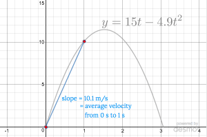
Now let's use those values to find the ball's average velocity for this interval: $a v e r a g e v e l o c i t y [0 s, 1.0 s] = 10.1 m ⏞ 𝑦 (1.0) - 0 m ⏞ 𝑦 (0) 1.0 - 0 = 10.1 - 0 1.0 = 10.1 m / s ✓$

Graph of the ball's position versus time, and the line segment connecting (0, y(0)) and (1, y(1)). The slope of that line segment equals the ball's average velocity for the interval, 10.1 m/s.

The average velocity equals the slope of the line segment that connects the points $(0, 𝑦 (0))$ and $(1, 𝑦 (1)),$ as shown in the figure.

You can also use the interactive Desmos graph at the bottom of this Example to see this value visually.

(b) To compute the ball's average velocity between $𝑡 = 2.0$ s and $𝑡 = 3.0$ s, we need its final position at $𝑡 2 = 3.0$ s and its initial position at $𝑡 1 = 2.0$ s. Let's again compute those first:

Quick subproblem to find $𝑦 (𝑡 2 = 3.0 s)$ and $𝑦 (𝑡 1 = 2.0 s)$ : $𝑦 (3.0 s) = 15 (3.0) - 4.9 (3.0) 2 = 0.9 m ◂ 𝑦 (2.0 s) = 15 (2.0) - 4.9 (2.0) 2 = 10.4 m ◂$

End quick subproblem.

Then the average velocity for this interval is:

a v e r a g e v e l o c i t y [2.0 s, 3.0 s] = 𝑦 (3.0) - 𝑦 (2.0) 3.0 - 2.0 = 0.9 - 10.4 1.0 = - 9.5 m / s ✓

$Tip icon$

Part (c) of the preceding example illustrates the same general conclusion we saw after considering Matt's swim on the preceding screen:

If the object begins and ends at the same location over an interval, then there is no change in position, and so its average velocity is zero for the interval.

While this result might seem odd, remember that average velocity doesn't focus on any of the details of the motion, and instead considers only the initial and final positions of the object and the duration of the interval. Hence an average velocity of zero tells you only that the object ends with with the same position where it began, and absolutely nothing about the motion that took place during the interval. Said differently, a ball that doesn't move at all, maintaining zero velocity throughout the motion, would begin and end its motion in the same position(s) as the ball that was shot upward. This is how average velocity is defined, and it's important that we all abide by this agreed-upon definition.

Practice, and Extension

Time for you to practice putting these ideas to deeper use. As we said above, these types of problems appear very frequently on exams, so please take this opportunity to make doing these types of calculations routine for yourself!

Practice Problem 1: Compute Average Velocity

The graph shows an object's position $𝑠,$ in meters, as a function of time $𝑡,$ in seconds.

Find the object's average velocity from $𝑡 = 0$ to $𝑡 = 10$ seconds.
Find the object's average velocity from $𝑡 = 10$ to $𝑡 = 30$ seconds.
Without doing any calculations, which is greater: the average velocity from 5 to 10 seconds, or the average velocity from 20 to 25 seconds? How can you tell?

Practice Problem #2: Better estimate of instantaneous velocity

Recall Example 3 above, "Approximate an object's velocity at an instant." We've now collected more data as shown in the table and accompanying graph.

𝑡 (s e c o n d s) 1.0 1.5 3.0 3.08 3.2 3.5 4.0 4.5 𝑠 (c m) 1.0 3.25 9.0 9.49 10.24 12.25 16 20.25

Use the data in the table to find a better approximation for the object's velocity at

𝑡 = 3.0

seconds.

(A) 6.125 c m s (B) 6.5 c m s (C) 3.83 c m s (D) 0 c m s (E) 6.0 c m s

ABCDE

Practice Problem #3: Cars Pass

Sandy is traveling on a straight road and is stopped at a red light. At exactly noon, the light turns green, and for the next bit of time her car's position is given by $𝑠 S a n d y (𝑡) = 1.5 𝑡 2 + 7$ where s is in meters (measured from a 0-kilometer marker on the road) and t is in seconds.

Michael is traveling at a constant rate on the same road, and passes Sandy exactly 2 seconds after noon. Since Sandy is accelerating, 4 seconds later, at 6 seconds after noon, Sandy passes Michael.

What is the constant speed of Michael's car, $𝑣 M i c h a e l$ ?

Hint: There's a close connection between finding Michael's constant speed and Sandy's average velocity. Do you see it? If not, tap "Open" here:

(A) 18.5 m s e c (B) 12 m s e c (C) 9.25 m s e c (D) 10.2 m s e c (E) n o n e o f t h e a b o v e

A B C D E

View/Hide Solution

We know that Michael is traveling at constant speed. We also know that his car is at the same position as Sandy's car at t = 2 sec, and at t = 6 sec. Hence we can calculate his constant speed, since we know his change in position is the same as Sandy's change in position over those 4 seconds. That is, Michael's constant speed is equal to Sandy's average velocity over this time interval: $𝑣 M i c h a e l = 𝑠 S a n d y (6 s e c) - 𝑠 S a n d y (2 s e c) 6 s e c - 2 s e c$ We need to calculate Sandy's car's position at $𝑡 = 6$ seconds: $𝑠 S a n d y (6) = 1.5 (6) 2 + 7 = 61 m ◂$ and at $𝑡 = 2$ seconds: $𝑠 S a n d y (2) = 1.5 (2) 2 + 7 = 13 m ◂$

Then $𝑣 M i c h a e l = 𝑣 a v g, S a n d y = 𝑠 S a n d y (6 s e c) - 𝑠 S a n d y (2 s e c) 6 s e c - 2 s e c = 61 m - 13 m 4 s e c = 48 m 4 s e c = 12 m s e c ✓$

Position versus time plots for Sandy and Michael. Sandy's motion starts at (0,7) and curves upward. Michael's motinon is an upward sloping line that intersects Sandy's curve at (2, s(2)) and (6, s(6)). The slope of Michael's line is shown: 12 m/sec.

Problem #3 nicely illustrates again the meaning of average velocity: If two objects start out together, and one travels at the constant speed equal to the other's average velocity over the chosen time-interval, then they will be at the same location again at the end of that interval.

Let's consider a problem that's more challenging to think through, but that draws on the same ideas. It's modeled on a question that appeared on a college-level exam.

Practice Problem #4: Sinusoid

The figure shows the x-position versus time graph of an object from

𝑡 = - 1.5

𝑡 = 7

. For how many values of

𝑎,

- 1 < 𝑎 < 7,

is the average velocity of the object equal to zero on the interval

[- 1, 𝑎] ?

(A) Z e r o (B) O n e (C) T w o (D) T h r e e (E) N e e d m o r e i n f o r m a t i o n

ABCDE

In the next topic we'll generalize the idea of average rate to apply to other quantities that change.

The Upshot

Average velocity over the interval $[𝑡 1, 𝑡 2]$ is defined by $a v e r a g e v e l o c i t y [𝑡 1, 𝑡 2] = c h a n g e i n p o s i t i o n c h a n g e i n t i m e = 𝑠 (𝑡 2) - 𝑠 (𝑡 1) 𝑡 2 - 𝑡 1$ where $𝑠 (𝑡 1)$ is the object's position at time $𝑡 1,$ and $𝑠 (𝑡 2)$ is its position at time $𝑡 2 .$
Average velocity over a time interval is the average rate of change of the object's position over that interval.
To obtain the best estimate possible of an object's instantaneous velocity at a particular moment from data in a table, use the smallest time interval around around that moment.

Questions or comments about anything on this screen? Pop over to the Forum and post!

B.2 Average Velocity Over Any Interval

Thinking about short time intervals, and initial "instantaneous velocity" estimates

Practice, and Extension

Thinking about short time intervals,
and initial "instantaneous velocity" estimates