A.3 Introducing Linear Approximations

On this screen we'll introduce one of the most important uses of Calculus: how to do a linear approximation. We'll learn how to quickly estimate something like $(3.01) 2$ , or $(0.99) 3 .$ Using Desmos interactive calculators will help us see how this works.

Deep Dive: Linear Approximation of $(3.01) 2$

Syd bikes up a hill of increasing steepness. A red dot on the center of his front tire indicates his position.

To start, recall that in the preceding Topic we considered the scenario of Syd biking up a curved path. As he passed the horizontal position $𝑥 = 3.00$ m, the path climbs at the rate $𝑑 𝑦 𝑑 𝑥 ∣ a t x = 3.00 m = 6.00 v e r t i c a l m h o r i z o n t a l m .$ With this information, we calculated the small change in his vertical position, dy, when he moved forward the small horizontal distance dx:

s m a l l c h a n g e i n v e r t p o s i t i o n = (r a t e a t h o r i z p o s i t i o n 𝑥 = 3.00 m) * (s m a l l c h a n g e i n h o r i z p o s i t i o n) 𝑑 𝑦 = (𝑑 𝑦 𝑑 𝑥 ∣ a t 𝑥 = 3.00 m) \cdot 𝑑 𝑥

And we calculated his vertical position after he had moved forward the small horizontal distance dx as

𝑦 v a l u e, a t 𝑥 + 𝑑 𝑥 ⏞ 𝑦 (𝑥 + 𝑑 𝑥) = 𝑦 v a l u e, a t 𝑥 ⏞ 𝑦 (𝑥) + (r a t e a t 𝑥) * 𝑑 𝑥 ⏞ ¯¯¯ ⏞ ¯¯¯ ⏞ s m a l l c h a n g e 𝑑 𝑦

Let's now consider a more mathematical example. Note that while the words may be different, the ideas and calculations are exactly the same as in that scenario. Keep the picture of Syd biking uphill in your mind as you consider the requested calculation.

Example 1: $𝑓 (𝑥) = 𝑥 2$

Graph of the function f(x) = x^2 for x > 0. Consider the function $𝑓 (𝑥) = 𝑥 2,$ graphed to the right.

You know that at $𝑥 = 3,$ $𝑓 (3) = 32 = 9 .$

For now, we'll simply tell you that the rate the function "climbs" at $𝑥 = 3$ is exactly 6: $𝑑 𝑓 𝑑 𝑥 ∣ a t x = 3.00 = 6$ (Later we'll show you how to determine this rate for yourself, a skill fundamental to Calculus. Activity 2 below will also address this value. For now, so you can start doing "real" Calculus calculations, let's just take the rate as a given.)

Use the information provided to find the (approximate) value of $𝑓 (3.01) .$
Hint: The calculation is exactly the same as finding Syd's vertical position $𝑦 (3.01) .$
Although the approximation will be less good for reasons we'll see, use the same approach to find the approximate value of $𝑓 (3.5) .$

Solution.

(a) Let's perform exactly the same calculation as we did to find Syd's change in vertical position. We know

𝑓 (3) = 9

and

𝑑 𝑓 𝑑 𝑥 ∣ a t x = 3.00 = 6,

and we have

𝑑 𝑥 = 0.01 .

So using the same formulation as before:

𝑓 v a l u e a t 𝑥 + 𝑑 𝑥 ⏞ 𝑓 (𝑥 + 𝑑 𝑥) = 𝑓 v a l u e a t 𝑥 ⏞ 𝑓 (𝑥) + (r a t e a t 𝑥) * 𝑑 𝑥 ⏞ ¯¯¯ ⏞ ¯¯¯ ⏞ s m a l l c h a n g e 𝑑 𝑓 𝑓 (3.01) = 𝑓 (3 + 0.01) = 𝑓 (3) + (6) \cdot (0.01) = 9 + 0.06 = 9.06 ✓

Note that the actual value is

𝑓 (3.01) = (3.01) 2 = 9.0601,

so this is a pretty great estimate for such a quick calculation! We'll discuss the tiny discrepancy between the values 9.06 and 9.0601 (a difference of 0.001%) below.

(b) The formulation for this calculation is the same, but now we have $𝑑 𝑥 = 0.5 :$ $𝑓 v a l u e a t 𝑥 + 𝑑 𝑥 ⏞ 𝑓 (𝑥 + 𝑑 𝑥) = 𝑓 v a l u e a t 𝑥 ⏞ 𝑓 (𝑥) + (r a t e a t 𝑥) * 𝑑 𝑥 ⏞ ¯¯¯ ⏞ ¯¯¯ ⏞ s m a l l c h a n g e 𝑑 𝑓 𝑓 (3.5) = 𝑓 (3 + 0.5) \approx 𝑓 (3) + (6) \cdot (0.5) \approx 9 + 3 \approx 12 ✓$ The actual value is $𝑓 (3.5) = (3.5) 2 = 12.25,$ so this is a less-good estimate than we made in (a). We'll discuss the larger discrepancy between the values 12 and 12.25 (a difference of 2%) immediately after this example.

Let's now use the following Activities to dig in and see why in Example 1 the approximation for $(3.01) 2$ works well and yet doesn't return the exact result, and why the approximation for $(3.5) 2$ works less well.

ACTIVITY 1.1: Zooming in on the curve $𝑦 = 𝑥 2$ around (3,9)

LINEAR APPROXIMATION: Replace a bit of the curve with an appropriate line

As the preceding Activity illustrates, we can approximate a curve's behavior by using the line instead, if we use an appropriate line, and if we stay within a region that is "close" to a particular point. Replacing a small section of a curve with a line of the correct slope in this way is known as a linear approximation. You can imagine that rather than walking along the curve itself, you're instead walking along this short line that mimics the curve's behavior. And we like lines, since they are much easier to work with than curves. The next activity shows how this super-handy replacement works mathematically.

ACTIVITY 1.2: Exploring the linear approximation

Graph showing the linear approximation for (3.01)^2: The curve is y=x^2, which looks like a line because we are zoomed-in so far. A triangle with lower left point (3,9) has base dx = 0.01, then vertically up with height df = 6(dx), shows how we go from the point (3,9) to the point (3.01, 9.06) since the slope of the line (hypotenuse) is given as 6.

We've seen thus far that our linear approximation method works by replacing a function's curve in a region around a specific point with a line that mimics the function's behavior at nearby points. The approach of course introduces some error, since we're following a line rather than the actual curve – and the farther we get from $𝑥 = 3,$ the more the line deviates from the curve.

Let's look more closely at this error that we introduce when using the linear approximation.

ACTIVITY 1.3: Explore the approximation error in dropping $(𝑑 𝑥) 2$

Deep Dive: Linear Approximation of $(0.99) 3$

Let's consider another example function, one for which we're dropping even more terms when we do our approximation.

Example 2: $𝑔 (𝑥) = 𝑥 3$

Consider the function $𝑔 (𝑥) = 𝑥 3,$ shown to the right.

You know that at $𝑥 = 1,$ $𝑔 (1) = (1) 3 = 1 .$

We are given that at $𝑥 = 1,$ the function changes at the rate $𝑑 𝑔 𝑑 𝑥 ∣ a t x = 1 = 3$

Using this information, find the approximate value of $(0.99) 3 .$

Solution.

We'll use exactly the same approach as we did for Syd's bike ride and as we did in Example 1. Note that this time dx is negative, $𝑑 𝑥 = - 0.01,$ since the x-value we're asked about, 0.99, is a little less than the value we know about at $𝑥 = 1$ .

𝑔 v a l u e a t 𝑥 + 𝑑 𝑥 ⏞ 𝑔 (𝑥 + 𝑑 𝑥) = 𝑔 v a l u e a t 𝑥 ⏞ 𝑔 (𝑥) + (r a t e a t 𝑥) * 𝑑 𝑥 ⏞ ¯¯¯ ⏞ ¯¯¯ ⏞ s m a l l c h a n g e 𝑑 𝑔 𝑔 (0.99) = 𝑔 (1 + (- 0.01)) \approx 𝑔 (1) + (3) \cdot (- 0.01) \approx 1 - 0.03 \approx 0.97 ✓

The actual value is $(0.99) 3 = 0.970299,$ a difference of 0.031%.

We'll once again expore the error between our linear approximation and the actual value in the next Activity.

ACTIVITY 2.1: Exploring the error in the linear approximation for $(0.99) 3$

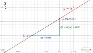
PART 1. Let's examine graphically the calculation we made in Example 2 above to find the approximation to $(0.99) 3$ . The interactive Desmos graph below shows the curve $𝑦 = 𝑥 3,$ with the point $(1, 1)$ highlighted.

Use the "+" button to zoom in, and drag the curve as needed to keep the point $(3, 9)$ near the center of the window.
When you have zoomed in sufficiently, you'll see a triangle appear with lines for dx and dg.
Use the slider beneath the graph to vary the value of dx.
Observe how for both positive and negative values of dx, the green line segment of the triangle closely tracks the red line of the function's curve.

PART 2. Let's again use some algebra to see why this linear approximation works. First, recall that

(𝑎 + 𝑏) 3 = 𝑎 3 + 3 𝑎 2 𝑏 + 3 𝑎 𝑏 2 + 𝑏 3

Since we have

𝑔 (𝑥) = 𝑥 3,

we can easily calculate the exact value of

𝑔 (0.99) = 𝑔 (1 + (- 0.01))

𝑔 (0.99) = 𝑔 (1 + (- 0.01)) = (1 + (- 0.01)) 3 = (1) 3 + 3 (1) 2 (- 0.01) + 3 (1) (- 0.01) 2 + (- 0.01) 3 = 1 - 3 (0.01) + 3 (0.0001) - 0.000001 = 1 - 0.03 + 0.0003 - 0.000001 = 0.970299

You can now see how our linear approximation works: we keep the first two terms of the above expression, and drop the third term,

3 (- 0.01) 2

, and the fourth term,

(- 0.01) 3)

, such that

𝑔 (0.99) \approx 1 - 0.03 = 0.97

And we quickly see that the approximation is off by only the small terms that we dropped.

More generally, for any value of dx we have

𝑔 (1 + 𝑑 𝑥) = (1 + 𝑑 𝑥) 3 = (1) 2 + 3 (1) 2 𝑑 𝑥 + 3 (1) (𝑑 𝑥) 2 + (𝑑 𝑥) 3 = 1 + 3 𝑑 𝑥 + 3 (𝑑 𝑥) 2 + (𝑑 𝑥) 3

Using our linear approximation approach, we drop the third,

3 (𝑑 𝑥) 2

term, and the fourth,

(𝑑 𝑥) 3

, term. This gives us an equation that depends linearly on dx:

𝑔 (1 + 𝑑 𝑥) \approx 1 + 3 𝑑 𝑥

By the way, by expanding the polynomial we once again just developed the rate of change for the function

𝑔 (𝑥) = 𝑥 3

𝑥 = 1

𝑑 𝑔 𝑑 𝑥 ∣ a t x = 1 = 3,

which is the multiplicative factor for the linear approximation here. We can again do this because we had a simple polynomial we could expand in

(1 + 𝑑 𝑥) 3 .

Remember that most functions do not allow for such an algebraic expansion, and so we still need to develop methods to determine the rate of change for any function we encounter.

The Examples and Activities above illustrate how linear approximations work: we keep only the linear term dx, which is known as the first-order term because it's dx to the first-power. By contrast, we drop all of the higher-order terms, here the second-order term, $(𝑑 𝑥) 2$ , and the third-order term, $(𝑑 𝑥) 3 .$ We'll learn much later in the course how to improve our approximations by including as many such higher-order terms as we'd like.

Time to practice some similar calculations for yourself! On the next screen you will find problems to practice with – each with a complete solution immediately available so you can easily check your work, or in case you need help. In the first problem you'll see how you can use our linear approximation method to estimate $\sqrt 16.2 .$

Have a question or comment about the super-cool ideas on this screen? We're getting to real Calculus now, based on the simple, everyday ideas you used on the preceding two screens. Please post your reactions and questions on our Forum!

The Upshot

For most functions $𝑓 (𝑥),$ if we know the value of the function at a particular value of x, and its rate of change $𝑑 𝑓 𝑑 𝑥 ∣ a t t h a t v a l u e o f x$ , then we can approximate the function's value a small interval dx away: $𝑓 (𝑥 + 𝑑 𝑥) \approx 𝑓 (𝑥) + 𝑑 𝑓 ⏞ ¯¯¯ ⏞ ¯¯¯ ⏞ (r a t e a t 𝑥) * 𝑑 𝑥$
This "linear approximation" method replaces the curve in the region close to the point we know about with a line segment that changes at the same rate as the original function at that point.
The linear approximation is a first-order approximation, since we keep the linear term dx but discard all higher-order terms (those involving $(𝑑 𝑥) 2,$ $(𝑑 𝑥) 3,$ and so forth).
The smaller the size of dx, the better the approximation is likely to be.

Don't wait: Start getting these ideas into your head, and hands, now by doing a related problem or two. It's all free, and of course the only way to learn something is by doing it for yourself!

A.3 Introducing Linear Approximations

Deep Dive: Linear Approximation of (3.01)2

Deep Dive: Linear Approximation of (0.99)3

Deep Dive: Linear Approximation of $(3.01) 2$

Deep Dive: Linear Approximation of $(0.99) 3$