D.1 Continuity at a Point and Over an Interval

We turn now to an idea closely related to limits, and a concept that we'll use often and need to define: "continuity." As you'll see, whether we can apply certain tools to a function at a given point requires that we know that the function is "continuous" there, so we need to understand what continuity is!

Your everyday sense of "continuity" is quite useful for thinking about continuity in mathematics and science: time sweeps along continuously; river water flows continuously; "I biked continuously for twenty miles without stopping." The key idea is that there is no interruption in something that is continuous — no gaps, leaps, or sudden breaks.

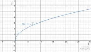
If you can draw the curve without lifting your pencil from the page, the function is continuous

We can translate these everyday ideas to a simple way to determine if a function is continuous by considering its graph: if you can draw a function's curve without lifting your pencil from the page, then that function is continuous. For example, each of the functions in the following figure is continuous:

By contrast, a function is not continuous if it has a jump or gap somewhere. We label such functions discontinuous, and there are examples in the figure below. Notice that for each of these functions you cannot draw the curve without lifting your pencil from the page. (The circle around the "hole" in the first graph of course actually indicates that the function is undefined there, and isn't actually a part of the function: if we were walking up along this line, we'd have to leap over that gap, which makes the function discontinuous. )

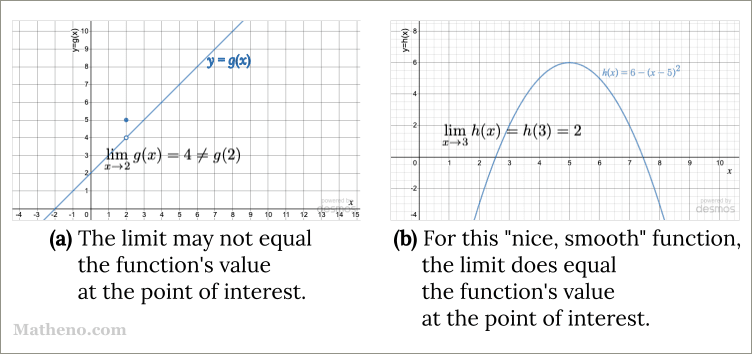
A more mathematical way to think about continuity is to notice that for a continuous function, if we make a small change in the function's input (imagine moving your hand a bit to the right as you draw the graph), the function's output changes by a small amount (so you don't have to suddenly move where your pencil is to draw the next bit). In fact, if a function is continuous at a particular point, then starting from that point you can make the function's change-in-output as small as you'd like by making the change-in-input sufficiently small.

By contrast, if the function is discontinuous at a point (like at 𝑥 =2 in each of the Discontinuous Example graphs above), then you cannot make the function's change in output as small as you'd like. Instead, the function's value on the left-side of the point is simply disconnected from its value on the right-side of the point.

The words, "make the change-in-output as small as you'd like by making the change-in-input sufficiently small" probably remind you of limits, as they should: the mathematical definition of "continuity" had to wait for the notion of "limit" to be developed, and relies heavily on that notion. Here is the official definition of Continuity at a Point:

First, for a function to be continuous at 𝑥 =𝑎 it must be defined there; otherwise there's automatically a "gap" of some sort, and so the function is discontinuous. But being defined at 𝑥 =𝑎 is not sufficient! For example in the bottom graph above, the function is defined at 𝑥 =2, but is clearly discontinuous at that point.

That bottom graph thus highlights the importance of the limit in the definition of continuity. Applying our understanding of limits from earlier, in words the definition says: a function is continuous at 𝑥 =𝑎 if the function is defined at 𝑥 =𝑎, and if we can make the the function's output 𝑓(𝑥) as close as we'd like to its value at 𝑥 =𝑎, 𝑓(𝑎), by making x sufficiently close to a. That is, using our 𝜖 and 𝛿 notation, we must be able to be within ±𝜖 of 𝑓(𝑎) ("as close as we'd like") by being within ±𝛿 of 𝑎 ("sufficiently close"). Kinda cool: see how important your understanding of the concept of "limits" is?

The Three Requirements for Continuity

As a practical matter, the continuity definition has three requirements. You should memorize these since an exam question about proving continuity automatically means that you must verify each of these:

Memorize these

1. 𝑓(𝑎) exists: a is in the domain of f.
2. lim𝑥→𝑎𝑓(𝑥) exists.
3. lim𝑥→𝑎𝑓(𝑥)=𝑓(𝑎): the limit equals the function's value at 𝑥 =𝑎.

You can see how each function in the Discontinuous Examples figure above fails one of the requirements: In the top two figures, the function is not defined at 𝑥 =2, and so we know immediately that the function is discontinuous there. (On an exam that's all you'd have to write; no need to proceed to the other items.) In the bottom graph, 𝑓(2) is defined so requirement #1 is fulfilled, but then lim𝑥→2𝑓(𝑥) does not exist and so the function is discontinuous at 𝑥 =2 by requirement #2. We'll of course let you practice showing that a function is continuous, or not, in problems below.

One-sided Continuity

Before then, let's introduce the idea of one-sided continuity, which is of course tied closely to the idea of one-sided limits. The figure to the right shows one of the example continuous functions from above, 𝑓(𝑥) =√𝑥. As we know, this function defined only for 𝑥 ≥0, and simply doesn't exist for 𝑥 <0. Its limit as 𝑥 →0 thus doesn't exist, and so we can't talk about its (general) continuity at 𝑥 =0. It is, however, "continuous from the right," meaning it satisfies the one-sided limit condition lim𝑥→0+=𝑓(0).

More generally, one-sided continuity at a point is defined by

Let's consider an example to show how this all works in practice.

Example 1: Semicircle continuous at endpoints

Consider the function 𝑓(𝑥) =√1−𝑥2, which has the domain [ −1,1]. Show that f is
(i) continuous from the right at the endpoint 𝑥 = −1, and
(ii) continuous from the left at 𝑥 =1.

Solution.

We use the Three Requirements for Continuity, now as applied for one-sided continuity:

(i) At 𝑥 = −1:

1. 𝑥 = −1 is in the domain of the function.
2. lim𝑥→−1+√1−𝑥2=√lim𝑥→−1+1−lim𝑥→−1+𝑥2=√1−1=0
   and so exists.
3. Since 𝑓( −1) =0, from 2.⏞¯¯¯¯⏞¯¯¯¯⏞lim𝑥→−1+√1−𝑥2=0=𝑓(−1).

Hence f is continuous from the right at 𝑥 = −1. ✓

(ii) At 𝑥 =1:

1. 𝑥 =1 is in the domain of the function.
2. lim𝑥→1−√1−𝑥2=√lim𝑥→1−1−lim𝑥→1−𝑥2=√1−1=0
   and so exists.
3. Since 𝑓(1) =0, from 2.⏞¯¯¯⏞¯¯¯⏞lim𝑥→1−√1−𝑥2=0=𝑓(1).

Hence f is continuous from the left at 𝑥 =1. ✓

Quick aside about Substitution and Continuity

The preceding example actually contains a subtle point: do you remember when we first introduced Substitution as a tactic for finding limits we said, rather informally, that we were looking at "a function that is defined at the point of interest and that behaves smoothly near the point of interest, meaning there are no jumps or gaps there"?

Open for reminder of discussion about Substitution to find a limit

Substitution to find a limit

When finding the limit lim𝑥→𝑎𝑓(𝑥), if you substitute 𝑥 =𝑎 into 𝑓(𝑥) and obtain a number for 𝑓(𝑎) (and don't get "undefined"), then the limit is simply that value 𝑓(𝑎): lim𝑥→𝑎𝑓(𝑥)=𝑓(𝑎)

As you saw in the examples above, when Substitution works you can find the limit easily, often in one line, which makes these problems quick. And we don't want to over-complicate that. At the same time, we want to emphasize again that lim𝑥→𝑎𝑓(𝑥) and 𝑓(𝑎) are two distinct quantities.

Recall our working definition of limits:

lim𝑥→𝑎𝑓(𝑥)=𝐿

is a number L (if one exists) such that 𝑓(𝑥) is as close to L as we want whenever x is sufficiently close to a.

We saw earlier various cases where lim𝑥→𝑎𝑓(𝑥)≠𝑓(𝑎) (figure (a), below). By contrast, for these "nice, smooth functions" the limit does simply equal 𝑓(𝑎) (figure (b) below).

collapse

We see now that what we were actually saying is that "if the function is continuous at 𝑥 =𝑎, then Substitution works." We thus didn't use Substitution to find the limit in requirement #2 in Example 1, since that would have assumed the very continuity that we're aiming to prove. (Instead, we invoked more formal limit laws and moved the limit inside the square-root symbol, and proceeded from there.) This is a subtle point, but worth mentioning.

Continuity is crucial: we can only use certain tools where a function is continuous

Indeed, very soon we'll see that we can only apply certain Calculus tools (like substitution, and later differentiation and integration) if a function is continuous. Going forward, rather than saying a function is "nice and smooth, with no gaps or jumps," we'll say simply "the function is continuous at 𝑥 =𝑎," or "if a function is continuous, then ...."

Everything above has focused on a function's continuity at a point. Let's now consider continuity over an interval of some sort:

Continuity on an Interval

Continuity on open intervals

No surprise: If the function f is continuous at every number in the open interval (𝑎,𝑏), then f is continuous on the interval (𝑎,𝑏).

Similarly, if it is continuous at every number in the infinite interval ( −∞,𝑏), (𝑎,∞), or ( −∞,∞), then it is continuous on that interval.

Continuity on closed intervals

We can extend these ideas to apply to continuity on a closed interval, simply by adding in the requirement that the function also be one-sided continuous at both endpoints of the interval:

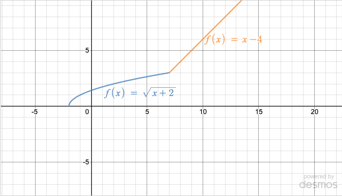
Example 1 (continued): Semicircle continuous over its entire domain

Consider again the function 𝑓(𝑥) =√1−𝑥2, which has the domain [ −1,1]. Show that f is continuous on its domain.

Solution.

To show that f is continuous on the open interval (1,1):

1. f is defined on this interval.
2. Consider an input-value 𝑥 =𝑐 in the interval −1 <𝑐 <1. Then lim𝑥→𝑐𝑓(𝑥)=√lim𝑥→𝑐1−lim𝑥→𝑐𝑥2=√1−𝑐2 and so exists.
3. Still thinking about 𝑥 =𝑐 in the same interval, since 𝑓(𝑐) =√1−𝑐2, from 2.⏞¯¯¯¯⏞¯¯¯¯⏞lim𝑥→𝑐𝑓(𝑥)=√1−𝑐2=𝑓(𝑐) Hence f is continuous at every 𝑥 =𝑐 in the interval ( −1,1). ◂

We already showed above in Example 1 that f is one-sided continuous at its endpoints 𝑥 = −1 and 𝑥 =1, and won't repeat the arguments here. Summarizing the results there, we have lim𝑥→1+𝑓(𝑥)=0=𝑓(−1)◂andlim𝑥→1−𝑓(𝑥)=0=𝑓(1)◂

Hence f is continuous on its entire domain [ −1,1]. ✓

Practice Problems: Continuity at a Point and Over an Interval

Time for some practice problems so you can consolidate the ideas here for yourself. Most students find problems that ask you to that a function is continuous a little awkward at first, but — as with most things — become less so with practice.

If you are going to be tested on continuity, make sure you know how to complete Problems #4 and #5, which are extremely common on exams.

Practice Problem 2

Let f be the function defined by 𝑓(𝑥)={√𝑥+2for −2≤𝑥≤7𝑥−4for 7<𝑥 Prove that f is, or is not, continuous at 𝑥 =7.

Reset Question

View/Hide Solution

To determine whether f is continuous or not, we simply step through the requirements and see whether the function satifies them all at 𝑥 =7 (in which case it's continuous there) or doesn't (in which case it's not). 𝑓(𝑥)={√𝑥+2for −2≤𝑥≤7𝑥−4for 7<𝑥 1. 𝑓(7) exists, and equals (note that for 𝑥 =7 we use the top equation) 𝑓(7)=√7+2=√9=3◂ 2. To determine whether the (general) limit exists for this piecewise function at 𝑥 =7, we must determine the limit from the left and from the right separately: lim𝑥→7−𝑓(𝑥)=lim𝑥→7−√𝑥+2=√9=3lim𝑥→7+𝑓(𝑥)=lim𝑥→7+(𝑥−4)=3 Hence lim𝑥→7−𝑓(𝑥)=lim𝑥→7+𝑓(𝑥)=3, and so the limit exists and lim𝑥→7𝑓(𝑥)=3 ◂
3. lim𝑥→7𝑓(𝑥)=3=𝑓(7)◂ and hence f is continuous at 𝑥 =7. ✓

The graph below shows how the two pieces of the function meet at 𝑥 =7, as we developed above.

The next few problems are typical exam questions.

On the next screen we'll give names to the different types of discontinuities, and see how to "remove a discontinuity." On the screen after that, we'll discuss continuous functions (including providing a list of functions that simply are continuous on their domains, which is super-helpful to know).

For now, what questions or comments do you have about the material on this screen, or any other Calculus concepts? Please join the discussion over on the Forum!

The Upshot

1. Informally, a function is continuous if you can draw its curve without lifting your pencil. Formally, a function f is continuous at 𝑥 =𝑎 if lim𝑥→𝑎𝑓(𝑥)=𝑓(𝑎)
2. To prove that a function is continuous at 𝑥 =𝑎, we must show three things (which you should memorize):
   1. 𝑓(𝑎) exists: a is in the domain of f.
   2. lim𝑥→𝑎𝑓(𝑥) exists.
   3. lim𝑥→𝑎𝑓(𝑥)=𝑓(𝑎): the limit equals the function's value at 𝑥 =𝑎.
3. For one-sided continuity, we consider only the limit from the left or from the right: Continuous from the right at 𝑥=𝑎:lim𝑥→𝑎+=𝑓(𝑎)Continuous from the left at 𝑥=𝑎:lim𝑥→𝑎−=𝑓(𝑎)
4. A function is continuous on the open interval (𝑎,𝑏) if it is continuous at every point in that interval. It is continuous on the closed interval [𝑎,𝑏] if it is continuous on the open interval (𝑎,𝑏) and also at the endpoints, such that lim𝑥→𝑎+𝑓(𝑥)=𝑓(𝑎)andlim𝑥→𝑏−𝑓(𝑥)=𝑓(𝑏)